Alpha Diversity
Last updated: 2020-06-17
Checks: 6 1
Knit directory: Fiber_Intervention_Study/
This reproducible R Markdown analysis was created with workflowr (version 1.6.2). The Checks tab describes the reproducibility checks that were applied when the results were created. The Past versions tab lists the development history.
The R Markdown file has unstaged changes. To know which version of the R Markdown file created these results, you’ll want to first commit it to the Git repo. If you’re still working on the analysis, you can ignore this warning. When you’re finished, you can run wflow_publish to commit the R Markdown file and build the HTML.
Great job! The global environment was empty. Objects defined in the global environment can affect the analysis in your R Markdown file in unknown ways. For reproduciblity it’s best to always run the code in an empty environment.
The command set.seed(20191210) was run prior to running the code in the R Markdown file. Setting a seed ensures that any results that rely on randomness, e.g. subsampling or permutations, are reproducible.
Great job! Recording the operating system, R version, and package versions is critical for reproducibility.
Nice! There were no cached chunks for this analysis, so you can be confident that you successfully produced the results during this run.
Great job! Using relative paths to the files within your workflowr project makes it easier to run your code on other machines.
Great! You are using Git for version control. Tracking code development and connecting the code version to the results is critical for reproducibility.
The results in this page were generated with repository version a16e6ef. See the Past versions tab to see a history of the changes made to the R Markdown and HTML files.
Note that you need to be careful to ensure that all relevant files for the analysis have been committed to Git prior to generating the results (you can use wflow_publish or wflow_git_commit). workflowr only checks the R Markdown file, but you know if there are other scripts or data files that it depends on. Below is the status of the Git repository when the results were generated:
Ignored files:
    Ignored:    .Rhistory
    Ignored:    .Rproj.user/
    Ignored:    code/.Rhistory
    Ignored:    reference-papers/Dietary_Variables.xlsx
    Ignored:    reference-papers/Johnson_2019.pdf
    Ignored:    renv/library/
    Ignored:    renv/staging/

Untracked files:
    Untracked:  analysis/glme_microbiome_genus_subset.Rmd
    Untracked:  analysis/glme_microbiome_phylum.Rmd
    Untracked:  analysis/microbiome_genus_prevotella_bacteroides.Rmd
    Untracked:  analysis/microbiome_genus_relative_abundance.Rmd
    Untracked:  data/analysis-data/DataDictionary_TOTALS_2018Record.xls
    Untracked:  fig/figure5_glmm_genus.pdf
    Untracked:  fig/figure5_glmm_phylum.pdf
    Untracked:  fig/misc/
    Untracked:  tab/results_glmm_microbiome_genus.csv
    Untracked:  tab/results_glmm_microbiome_phylum.csv
    Untracked:  tab/tables_results_2020-06-08.zip
    Untracked:  tab/tables_results_2020-06-08/

Unstaged changes:
    Modified:   analysis/alpha_diversity.Rmd
    Modified:   analysis/data_processing.Rmd
    Deleted:    analysis/glme_microbiome.Rmd
    Modified:   analysis/index.Rmd
    Modified:   analysis/microbiome_diet_trends.Rmd
    Modified:   code/get_cleaned_data.R
    Modified:   code/microbiome_statistics_and_functions.R
    Deleted:    fig/figure2.pdf
    Modified:   fig/figure2_individual_beta_diversity_over_study.pdf
    Deleted:    fig/figure3.pdf
    Modified:   fig/figure3_PCoA_analysis_results_beta_diversity_between_groups.pdf
    Deleted:    fig/figure4.pdf
    Modified:   fig/figure4_final_microbiome_diet_variables_over_time.pdf
    Modified:   fig/figure4_legend.pdf
    Deleted:    fig/figure5_glmm.pdf
    Deleted:    fig/figures-2020-06-08.zip
    Deleted:    fig/glmm_res.pdf
    Deleted:    fig/glmm_res.png
    Deleted:    fig/microbiome_abundance_glmm_results.pdf
    Deleted:    fig/predicted_Actinobacteria.png
    Deleted:    fig/predicted_Actinobacteria_model0.png
    Deleted:    fig/predicted_Actinobacteria_model1.png
    Deleted:    fig/predicted_Actinobacteria_model2.png
    Deleted:    fig/predicted_Actinobacteria_model3.png
    Deleted:    fig/predicted_Actinobacteria_model4.png
    Deleted:    fig/predicted_Actinobacteria_model5.png
    Deleted:    fig/predicted_Actinobacteria_model6.png
    Deleted:    fig/predicted_Actinobacteria_model7.png
    Deleted:    fig/predicted_Bacteroidetes.png
    Deleted:    fig/predicted_Bacteroidetes_model0.png
    Deleted:    fig/predicted_Bacteroidetes_model1.png
    Deleted:    fig/predicted_Bacteroidetes_model2.png
    Deleted:    fig/predicted_Bacteroidetes_model3.png
    Deleted:    fig/predicted_Bacteroidetes_model4.png
    Deleted:    fig/predicted_Bacteroidetes_model5.png
    Deleted:    fig/predicted_Bacteroidetes_model6.png
    Deleted:    fig/predicted_Bacteroidetes_model7.png
    Deleted:    fig/predicted_Cyanobacteria.png
    Deleted:    fig/predicted_Cyanobacteria_model0.png
    Deleted:    fig/predicted_Cyanobacteria_model1.png
    Deleted:    fig/predicted_Cyanobacteria_model2.png
    Deleted:    fig/predicted_Cyanobacteria_model3.png
    Deleted:    fig/predicted_Cyanobacteria_model4.png
    Deleted:    fig/predicted_Cyanobacteria_model5.png
    Deleted:    fig/predicted_Cyanobacteria_model6.png
    Deleted:    fig/predicted_Cyanobacteria_model7.png
    Deleted:    fig/predicted_Euryarchaeota.png
    Deleted:    fig/predicted_Euryarchaeota_model0.png
    Deleted:    fig/predicted_Euryarchaeota_model1.png
    Deleted:    fig/predicted_Euryarchaeota_model2.png
    Deleted:    fig/predicted_Euryarchaeota_model3.png
    Deleted:    fig/predicted_Euryarchaeota_model4.png
    Deleted:    fig/predicted_Euryarchaeota_model5.png
    Deleted:    fig/predicted_Euryarchaeota_model6.png
    Deleted:    fig/predicted_Euryarchaeota_model7.png
    Deleted:    fig/predicted_Firmicutes.png
    Deleted:    fig/predicted_Firmicutes_model0.png
    Deleted:    fig/predicted_Firmicutes_model1.png
    Deleted:    fig/predicted_Firmicutes_model2.png
    Deleted:    fig/predicted_Firmicutes_model3.png
    Deleted:    fig/predicted_Firmicutes_model4.png
    Deleted:    fig/predicted_Firmicutes_model5.png
    Deleted:    fig/predicted_Firmicutes_model6.png
    Deleted:    fig/predicted_Firmicutes_model7.png
    Deleted:    fig/predicted_Fusobacteria.png
    Deleted:    fig/predicted_Fusobacteria_model0.png
    Deleted:    fig/predicted_Fusobacteria_model1.png
    Deleted:    fig/predicted_Fusobacteria_model2.png
    Deleted:    fig/predicted_Fusobacteria_model3.png
    Deleted:    fig/predicted_Fusobacteria_model4.png
    Deleted:    fig/predicted_Fusobacteria_model5.png
    Deleted:    fig/predicted_Fusobacteria_model6.png
    Deleted:    fig/predicted_Fusobacteria_model7.png
    Deleted:    fig/predicted_Lentisphaerae.png
    Deleted:    fig/predicted_Lentisphaerae_model0.png
    Deleted:    fig/predicted_Lentisphaerae_model1.png
    Deleted:    fig/predicted_Lentisphaerae_model2.png
    Deleted:    fig/predicted_Lentisphaerae_model3.png
    Deleted:    fig/predicted_Lentisphaerae_model4.png
    Deleted:    fig/predicted_Lentisphaerae_model5.png
    Deleted:    fig/predicted_Lentisphaerae_model6.png
    Deleted:    fig/predicted_Lentisphaerae_model7.png
    Deleted:    fig/predicted_Proteobacteria.png
    Deleted:    fig/predicted_Proteobacteria_model0.png
    Deleted:    fig/predicted_Proteobacteria_model1.png
    Deleted:    fig/predicted_Proteobacteria_model2.png
    Deleted:    fig/predicted_Proteobacteria_model3.png
    Deleted:    fig/predicted_Proteobacteria_model4.png
    Deleted:    fig/predicted_Proteobacteria_model5.png
    Deleted:    fig/predicted_Proteobacteria_model6.png
    Deleted:    fig/predicted_Proteobacteria_model7.png
    Deleted:    fig/predicted_Tenericutes.png
    Deleted:    fig/predicted_Tenericutes_model0.png
    Deleted:    fig/predicted_Tenericutes_model1.png
    Deleted:    fig/predicted_Tenericutes_model2.png
    Deleted:    fig/predicted_Tenericutes_model3.png
    Deleted:    fig/predicted_Tenericutes_model4.png
    Deleted:    fig/predicted_Tenericutes_model5.png
    Deleted:    fig/predicted_Tenericutes_model6.png
    Deleted:    fig/predicted_Tenericutes_model7.png
    Deleted:    fig/predicted_Verrucomicrobia.png
    Deleted:    fig/predicted_Verrucomicrobia_model0.png
    Deleted:    fig/predicted_Verrucomicrobia_model1.png
    Deleted:    fig/predicted_Verrucomicrobia_model2.png
    Deleted:    fig/predicted_Verrucomicrobia_model3.png
    Deleted:    fig/predicted_Verrucomicrobia_model4.png
    Deleted:    fig/predicted_Verrucomicrobia_model5.png
    Deleted:    fig/predicted_Verrucomicrobia_model6.png
    Deleted:    fig/predicted_Verrucomicrobia_model7.png
Note that any generated files, e.g. HTML, png, CSS, etc., are not included in this status report because it is ok for generated content to have uncommitted changes.
These are the previous versions of the repository in which changes were made to the R Markdown (analysis/alpha_diversity.Rmd) and HTML (docs/alpha_diversity.html) files. If you’ve configured a remote Git repository (see ?wflow_git_remote), click on the hyperlinks in the table below to view the files as they were in that past version.
| File | Version | Author | Date | Message |
|---|---|---|---|---|
| html | 9da43aa | noah-padgett | 2020-06-08 | Build site. |
| Rmd | 774d405 | noah-padgett | 2020-06-01 | updated glmm and figures |
| html | 774d405 | noah-padgett | 2020-06-01 | updated glmm and figures |
| html | 0733fe5 | noah-padgett | 2020-05-21 | Build site. |
| Rmd | 036301e | noah-padgett | 2020-02-27 | updated alpha analysis |
| html | 036301e | noah-padgett | 2020-02-27 | updated alpha analysis |
| html | 51b6275 | noah-padgett | 2020-02-20 | Build site. |
| Rmd | 1c719ff | noah-padgett | 2020-02-20 | updated output window size |
| html | 1c719ff | noah-padgett | 2020-02-20 | updated output window size |
| html | c1bce73 | noah-padgett | 2019-12-11 | Build site. |
| Rmd | db73f64 | noah-padgett | 2019-12-11 | alpha diversity initial analysis |
| html | db73f64 | noah-padgett | 2019-12-11 | alpha diversity initial analysis |
This page contains the investigation of alpha diversity investigations.
Alpha diversity
Boxplots by unique participants
Observed OTUs
p <- ggplot(plot_data, aes(x=SubjectID10, y=Observed,
                      colour=SubjectID10, shape=Week))+
  geom_point(size=3) +
  facet_grid(.~Intervention2, scales = "free")+
  labs(x="Subject ID", y= "Observed OTUs")+
  guides(colour= guide_legend(title = "Subject ID"))+
  theme(panel.grid = element_blank(),
        strip.text.x = element_text(angle = 0, size = 11, face = "italic"),
        axis.text.y = element_text(size = 10),
        axis.title = element_text(size = 10),
        plot.title = element_text(hjust = 0.5),
        axis.title.x = element_blank(),
        strip.background = element_blank(),
        legend.position = "right",
        #legend.text = element_text(size = 7),
        #legend.title = element_blank(),
        panel.spacing.x=unit(0.001, "lines"))
p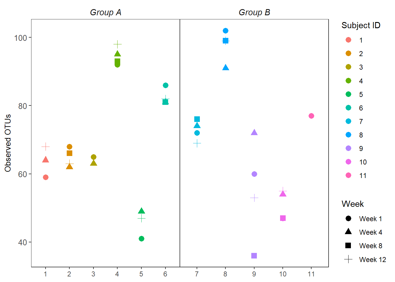
#ggsave("fig/figure1.pdf", p, width=5, height=3.5, units="in")Shannon Index
p <- ggplot(plot_data, aes(x=SubjectID10, y=Shannon,
                      colour=SubjectID10, shape=Week))+
  geom_point(size=3) +
  facet_grid(.~Intervention2, scales = "free")+
  labs(x="Subject ID", y= "Shannon Index")+
  guides(colour= guide_legend(title = "Subject ID"))+
  theme(panel.grid = element_blank(),
        strip.text.x = element_text(angle = 0, size = 11, face = "italic"),
        axis.text.y = element_text(size = 10),
        axis.title = element_text(size = 10),
        plot.title = element_text(hjust = 0.5),
        axis.title.x = element_blank(),
        strip.background = element_blank(),
        legend.position = "right",
        #legend.text = element_text(size = 7),
        #legend.title = element_blank(),
        panel.spacing.x=unit(0.001, "lines"))
p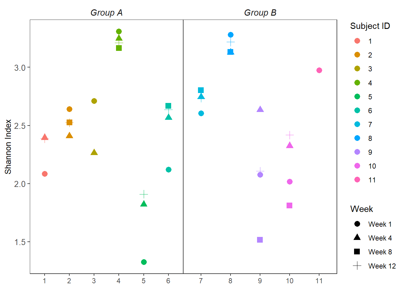
Simpson
p <- ggplot(plot_data, aes(x=SubjectID10, y=Simpson,
                      colour=SubjectID10, shape=Week))+
  geom_point(size=3) +
  facet_grid(.~Intervention2, scales = "free")+
  labs(x="Subject ID", y= "Simpson Index")+
  guides(colour= guide_legend(title = "Subject ID"))+
  theme(panel.grid = element_blank(),
        strip.text.x = element_text(angle = 0, size = 11, face = "italic"),
        axis.text.y = element_text(size = 10),
        axis.title = element_text(size = 10),
        plot.title = element_text(hjust = 0.5),
        axis.title.x = element_blank(),
        strip.background = element_blank(),
        legend.position = "right",
        #legend.text = element_text(size = 7),
        #legend.title = element_blank(),
        panel.spacing.x=unit(0.001, "lines"))
p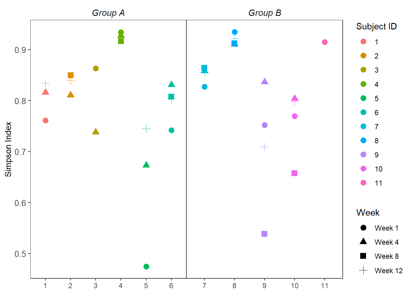
Inverse Simpson
p <- ggplot(plot_data, aes(x=SubjectID10, y=InvSimpson,
                      colour=SubjectID10, shape=Week))+
  geom_point(size=3) +
  facet_grid(.~Intervention2, scales = "free")+
  labs(x="Subject ID", y= "Inverse Simpson Index")+
  guides(colour= guide_legend(title = "Subject ID"))+
  theme(panel.grid = element_blank(),
        strip.text.x = element_text(angle = 0, size = 11, face = "italic"),
        axis.text.y = element_text(size = 10),
        axis.title = element_text(size = 10),
        plot.title = element_text(hjust = 0.5),
        axis.title.x = element_blank(),
        strip.background = element_blank(),
        legend.position = "right",
        #legend.text = element_text(size = 7),
        #legend.title = element_blank(),
        panel.spacing.x=unit(0.001, "lines"))
p
Boxplots by week of study
Observed OTUs
p <- ggplot(plot_data, aes(x=Intervention, y=Observed,
                            colour=Intervention,
                            group=Intervention))+
  geom_boxplot(outlier.shape=NA)+
  geom_point(size=3, position="jitter")+
  facet_wrap(.~Week, nrow=1)+
  labs(x=NULL, y="Observed OTUs",
       title="Observed OTUs by Study Week")+
  guides(colour= guide_legend(title = "Intervention"))+
  scale_colour_manual(values = cols)+
  theme(panel.grid = element_blank(),
        strip.text.x = element_text(angle = 0, size = 11, face = "italic"),
        axis.text.y = element_text(size = 10),
        axis.title = element_text(size = 10),
        plot.title = element_text(hjust = 0.5),
        axis.title.x = element_blank(),
        strip.background = element_blank(),
        legend.position = "right",
        #legend.text = element_text(size = 7),
        #legend.title = element_blank(),
        panel.spacing.x=unit(0.001, "lines"))
p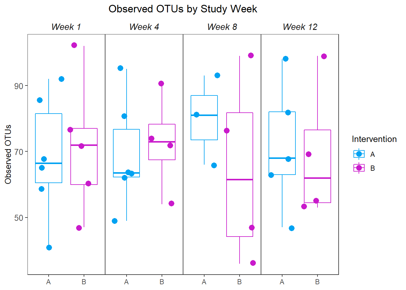
Shannon Index
p <- ggplot(plot_data, aes(x=Intervention, y=Shannon,
                            colour=Intervention,
                            group=Intervention))+
  geom_boxplot(outlier.shape=NA)+
  geom_point(size=3, position="jitter")+
  facet_wrap(.~Week, nrow=1)+
  labs(x=NULL, y="Shannon Index",
       title="Shannon Index by Study Week")+
  guides(colour= guide_legend(title = "Intervention"))+
  scale_colour_manual(values = cols)+
  theme(panel.grid = element_blank(),
        strip.text.x = element_text(angle = 0, size = 11, face = "italic"),
        axis.text.y = element_text(size = 10),
        axis.title = element_text(size = 10),
        plot.title = element_text(hjust = 0.5),
        axis.title.x = element_blank(),
        strip.background = element_blank(),
        legend.position = "right",
        #legend.text = element_text(size = 7),
        #legend.title = element_blank(),
        panel.spacing.x=unit(0.001, "lines"))
p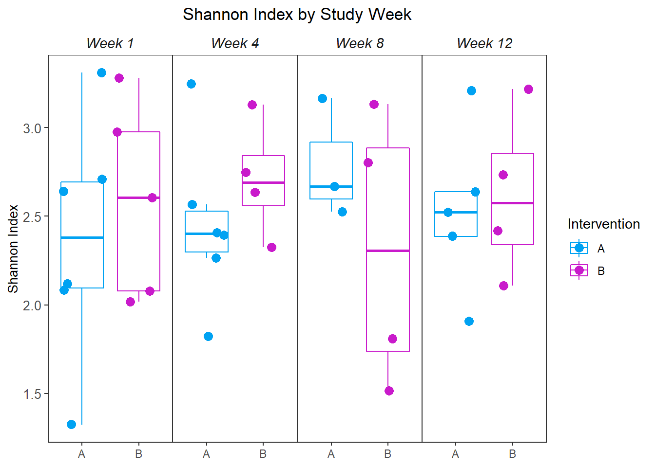
Simpson
p <- ggplot(plot_data, aes(x=Intervention, y=Simpson,
                            colour=Intervention,
                            group=Intervention))+
  geom_boxplot(outlier.shape=NA)+
  geom_point(size=3, position="jitter")+
  facet_wrap(.~Week, nrow=1)+
  labs(x=NULL, y="Simpson",
       title="Simpson by Study Week")+
  guides(colour= guide_legend(title = "Intervention"))+
  scale_colour_manual(values = cols)+
  theme(panel.grid = element_blank(),
        strip.text.x = element_text(angle = 0, size = 11, face = "italic"),
        axis.text.y = element_text(size = 10),
        axis.title = element_text(size = 10),
        plot.title = element_text(hjust = 0.5),
        axis.title.x = element_blank(),
        strip.background = element_blank(),
        legend.position = "right",
        #legend.text = element_text(size = 7),
        #legend.title = element_blank(),
        panel.spacing.x=unit(0.001, "lines"))
p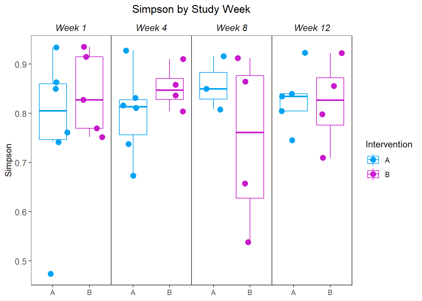
Inverse Simpson
p <- ggplot(plot_data, aes(x=Intervention, y=InvSimpson,
                            colour=Intervention,
                            group=Intervention))+
  geom_boxplot(outlier.shape=NA)+
  geom_point(size=3, position="jitter")+
  facet_wrap(.~Week, nrow=1)+
  labs(x=NULL, y="Inverse Simpson",
       title="Inverse Simpson by Study Week")+
  guides(colour= guide_legend(title = "Intervention"))+
  scale_colour_manual(values = cols)+
  theme(panel.grid = element_blank(),
        strip.text.x = element_text(angle = 0, size = 11, face = "italic"),
        axis.text.y = element_text(size = 10),
        axis.title = element_text(size = 10),
        plot.title = element_text(hjust = 0.5),
        axis.title.x = element_blank(),
        strip.background = element_blank(),
        legend.position = "right",
        #legend.text = element_text(size = 7),
        #legend.title = element_blank(),
        panel.spacing.x=unit(0.001, "lines"))
p
Manuscript Figure
p1 <- ggplot(plot_data, aes(x=SubjectID10, y=Observed,
                      colour=SubjectID10, shape=Week))+
  geom_point(size=3) +
  facet_grid(.~Intervention2, scales = "free")+
  labs(x="Subject ID", y= "Observed OTUs",
       title="Observed OTUs by Participants")+
  guides(colour= guide_legend(title = "Subject ID"))+
  scale_colour_manual(values = cols)+
  theme(panel.grid = element_blank(),
        strip.text.x = element_text(angle = 0, size = 11, face = "italic"),
        axis.text.y = element_text(size = 10),
        axis.title = element_text(size = 10),
        plot.title = element_text(hjust = 0.5),
        axis.title.x = element_blank(),
        strip.background = element_blank(),
        legend.position = "right",
        #legend.text = element_text(size = 7),
        #legend.title = element_blank(),
        panel.spacing.x=unit(0.001, "lines"))
p1
p2 <- ggplot(plot_data, aes(x=Intervention, y=Observed,
                            colour=Intervention,
                            group=Intervention))+
  geom_boxplot(outlier.shape=NA)+
  geom_point(size=3, position="jitter")+
  facet_wrap(.~Week, nrow=1)+
  labs(x=NULL, y="Observed OTUs",
       title="Observed OTUs by Study Week")+
  guides(colour= guide_legend(title = "Intervention"))+
  scale_colour_manual(values = cols)+
  theme(panel.grid = element_blank(),
        strip.text.x = element_text(angle = 0, size = 11, face = "italic"),
        axis.text.y = element_text(size = 10),
        axis.title = element_text(size = 10),
        plot.title = element_text(hjust = 0.5),
        axis.title.x = element_blank(),
        strip.background = element_blank(),
        legend.position = "right",
        #legend.text = element_text(size = 7),
        #legend.title = element_blank(),
        panel.spacing.x=unit(0.001, "lines"))
p2 
p3 <- ggplot(plot_data, aes(x=SubjectID10, y=Shannon,
                      colour=SubjectID10, shape=Week))+
  geom_point(size=3) +
  facet_grid(.~Intervention2, scales = "free")+
  labs(x="Subject ID", y= "Shannon Index",
       title="Shannon Index by Participants")+
  guides(colour= guide_legend(title = "Subject ID"))+
  scale_colour_manual(values = cols)+
  theme(panel.grid = element_blank(),
        strip.text.x = element_text(angle = 0, size = 11, face = "italic"),
        axis.text.y = element_text(size = 10),
        axis.title = element_text(size = 10),
        plot.title = element_text(hjust = 0.5),
        axis.title.x = element_blank(),
        strip.background = element_blank(),
        legend.position = "right",
        #legend.text = element_text(size = 7),
        #legend.title = element_blank(),
        panel.spacing.x=unit(0.001, "lines"))
p3
p4 <- ggplot(plot_data, aes(x=Intervention, y=Shannon,
                            colour=Intervention,
                            group=Intervention))+
  geom_boxplot(outlier.shape=NA)+
  geom_point(size=3, position="jitter")+
  facet_wrap(.~Week, nrow=1)+
  labs(x=NULL, y="Shannon Index",
       title="Shannon Index by Study Week")+
  guides(colour= guide_legend(title = "Intervention"))+
  scale_colour_manual(values = cols)+
  theme(panel.grid = element_blank(),
        strip.text.x = element_text(angle = 0, size = 11, face = "italic"),
        axis.text.y = element_text(size = 10),
        axis.title = element_text(size = 10),
        plot.title = element_text(hjust = 0.5),
        axis.title.x = element_blank(),
        strip.background = element_blank(),
        legend.position = "right",
        #legend.text = element_text(size = 7),
        #legend.title = element_blank(),
        panel.spacing.x=unit(0.001, "lines"))
p4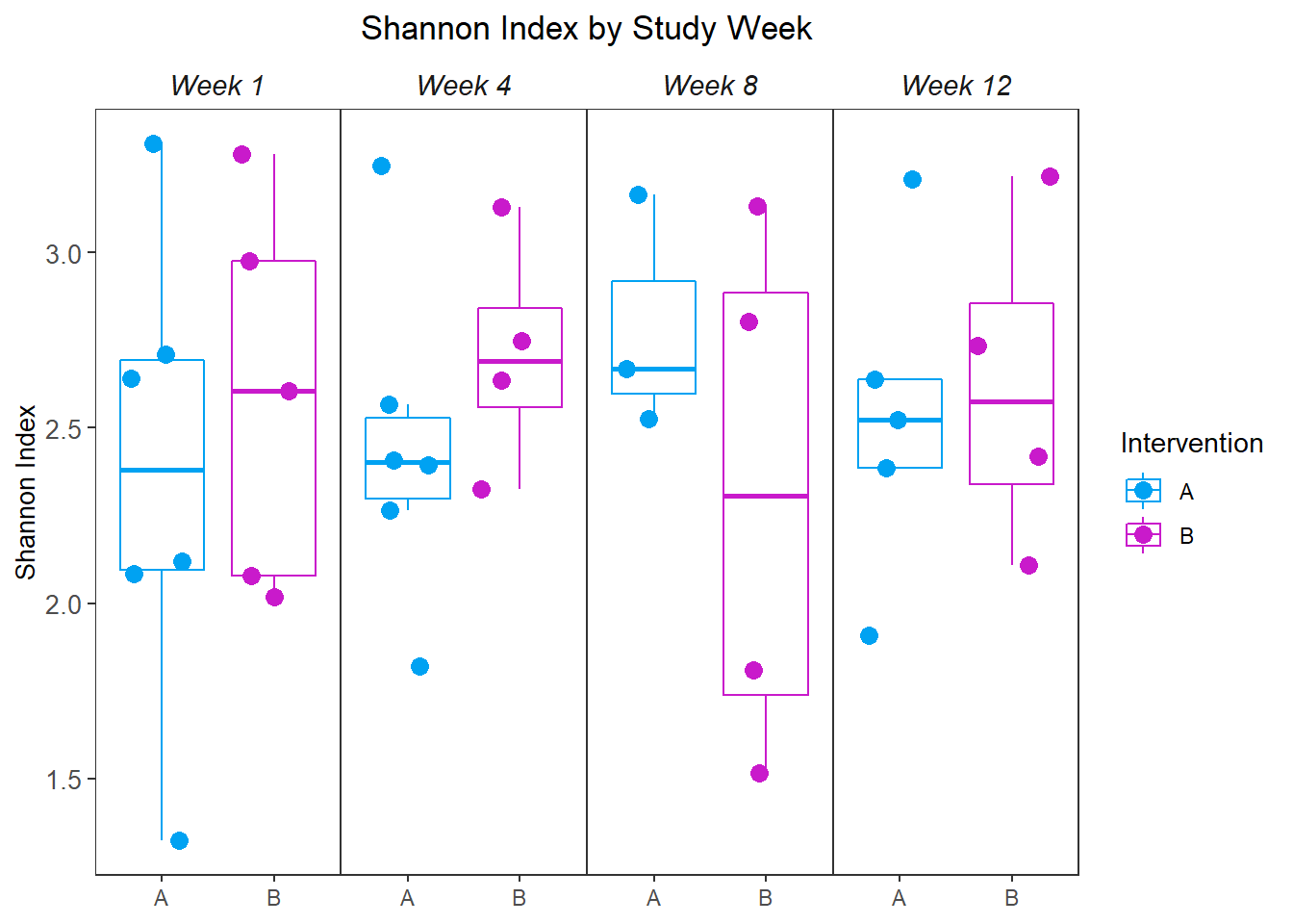
p5 <- ggplot(plot_data, aes(x=SubjectID10, y=InvSimpson,
                      colour=SubjectID10, shape=Week))+
  geom_point(size=3) +
  facet_grid(.~Intervention2, scales = "free")+
  labs(x="Subject ID", y= "Inverse Simpson",
       title="Inverse Simpson by Participants")+
  guides(colour= guide_legend(title = "Subject ID"))+
  scale_colour_manual(values = cols)+
  theme(panel.grid = element_blank(),
        strip.text.x = element_text(angle = 0, size = 11, face = "italic"),
        axis.text.y = element_text(size = 10),
        axis.title = element_text(size = 10),
        plot.title = element_text(hjust = 0.5),
        axis.title.x = element_blank(),
        strip.background = element_blank(),
        legend.position = "right",
        #legend.text = element_text(size = 7),
        #legend.title = element_blank(),
        panel.spacing.x=unit(0.001, "lines"))
p5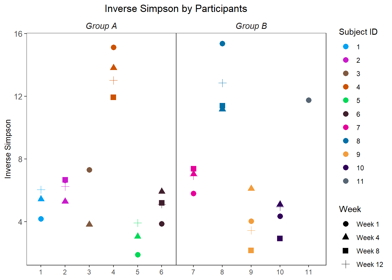
p6 <- ggplot(plot_data, aes(x=Intervention, y=InvSimpson,
                            colour=Intervention,
                            group=Intervention))+
  geom_boxplot(outlier.shape=NA)+
  geom_point(size=3, position="jitter")+
  facet_wrap(.~Week, nrow=1)+
  labs(x=NULL, y="Inverse Simpson",
       title="Inverse Simpson by Study Week")+
  guides(colour= guide_legend(title = "Intervention"))+
  scale_colour_manual(values = cols)+
  theme(panel.grid = element_blank(),
        strip.text.x = element_text(angle = 0, size = 11, face = "italic"),
        axis.text.y = element_text(size = 10),
        axis.title = element_text(size = 10),
        plot.title = element_text(hjust = 0.5),
        axis.title.x = element_blank(),
        strip.background = element_blank(),
        legend.position = "right",
        #legend.text = element_text(size = 7),
        #legend.title = element_blank(),
        panel.spacing.x=unit(0.001, "lines"))
p6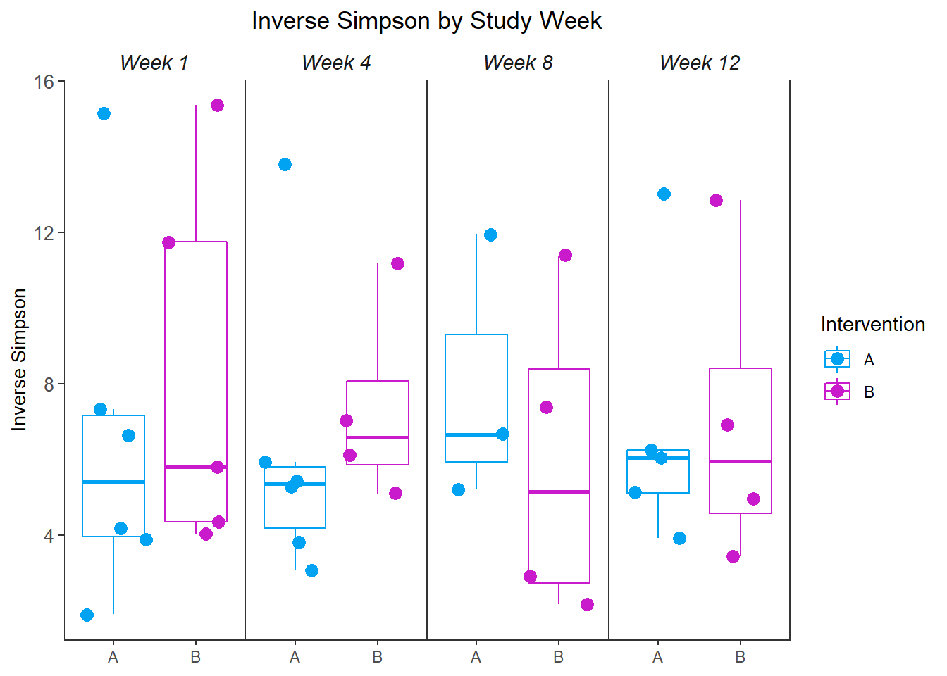
  library(cowplot)
  p1.leg <- get_legend(p1)
  p2.leg <- get_legend(p2)

  p1.nl <- p1 + theme(legend.position = "none", plot.title = element_blank(), axis.text.x = element_blank(), axis.ticks.x = element_blank())
  p2.nl <- p2 + theme(legend.position = "none", plot.title = element_blank(), axis.text.y = element_blank(),axis.text = element_blank(), axis.title = element_blank(), axis.ticks = element_blank())
  p3.nl <- p3 + theme(legend.position = "none", plot.title = element_blank(), axis.text.x = element_blank(), axis.ticks.x = element_blank(), strip.text.x = element_blank())
  p4.nl <- p4 + theme(legend.position = "none", plot.title = element_blank(), axis.text.y = element_blank(), axis.text.x = element_blank(), axis.title.y = element_blank(), axis.ticks = element_blank(), strip.text.x = element_blank())
  p5.nl <- p5 + theme(plot.title =  element_blank(), strip.text.x = element_blank(), legend.position="none")
  p6.nl <- p6 + theme(plot.title = element_blank(), axis.text.y = element_blank(), axis.title.y = element_blank(), axis.ticks.y = element_blank(), strip.text.x = element_blank(), legend.position="none")

  p <- p1.nl +  p2.nl + p3.nl + p4.nl + p5.nl + p6.nl + plot_layout(nrow=3, ncol=2)
  p
  ggsave("fig/figure1.pdf", p, width=7.9,height=5, units="in")


  #bigplotlegend <- plot_grid(p1.leg, p2.leg, nrow =1, align = "h")

  #save_plot("fig/figure1_legend.pdf", bigplotlegend, base_width = 13.25, base_height = 5)
Intervention Effect
Overall Effect
Observed OTUs
ggplot(plot_data, aes(x=Intervention, y=Observed))+
  geom_boxplot(outlier.alpha = 0,
               aes(group=Intervention, color=Intervention))+
  geom_point(position="jitter",aes(color=Intervention))+
  guides(colour= guide_legend(title = "Intervention"))+
  labs(x="Intervention Group")+
  theme(axis.text.x = element_text(angle = 0, hjust=0.33))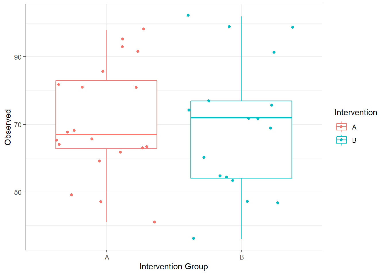
Shannon Index
ggplot(plot_data, aes(x=Intervention, y=Shannon))+
  geom_boxplot(outlier.alpha = 0,
               aes(group=Intervention, color=Intervention))+
  geom_point(position="jitter",aes(color=Intervention))+
  guides(colour= guide_legend(title = "Intervention"))+
  labs(x="Intervention Group")+
  theme(axis.text.x = element_text(angle = 0, hjust=0.33))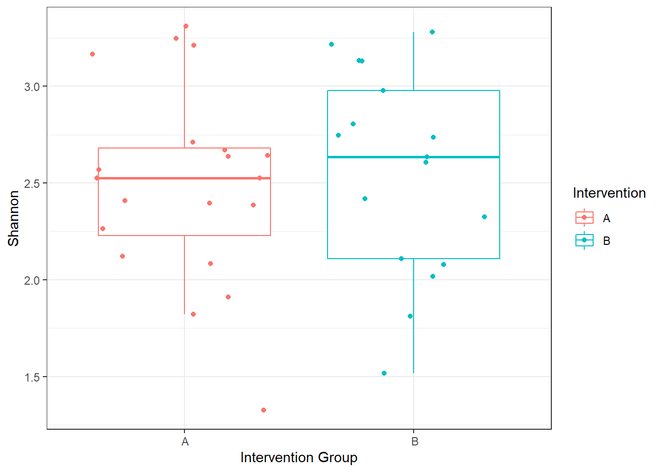
Simpson
ggplot(plot_data, aes(x=Intervention, y=Simpson))+
  geom_boxplot(outlier.alpha = 0,aes(group=Intervention, color=Intervention))+
  geom_point(position="jitter",aes(color=Intervention))+
  guides(colour= guide_legend(title = "Intervention"))+
  labs(x="Intervention Group")+
  theme(axis.text.x = element_text(angle = 0, hjust=0.33))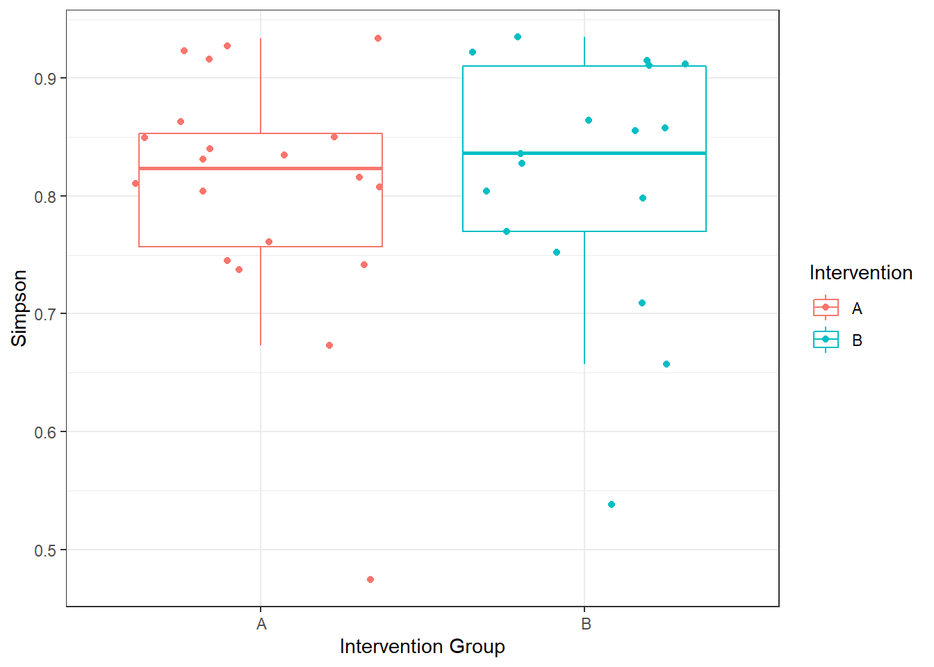
Changes Over Time
Observed OTUs
ggplot(plot_data, aes(x=Intervention, y=Observed,
                      group=Intervention,
                      color=Intervention, shape=Intervention))+
  geom_boxplot(outlier.alpha = 0)+
  geom_point(position="jitter")+
  facet_grid(.~Week)+
  labs(x="Intervention Group by Week")+
  guides(colour= guide_legend(title = "Intervention"))+
  theme(axis.text.x = element_text(angle = 0, hjust=0.33))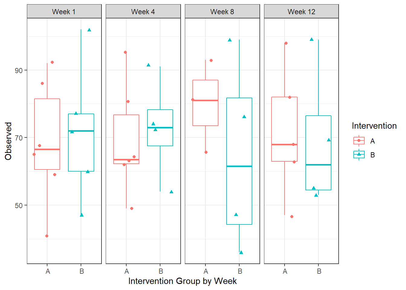
ggplot(plot_data, aes(x=Week, y=Observed,
                      group=interaction(Intervention, SubjectID3),
                      color=SubjectID3, shape=Intervention))+
  #geom_boxplot(outlier.alpha = 0)+
  geom_point()+
  geom_line()+
  #facet_grid(.~Week)+
  labs(x="Intervention Group by Week")+
  guides(colour= guide_legend(title = "Intervention"))+
  theme(axis.text.x = element_text(angle = 0, hjust=0.33))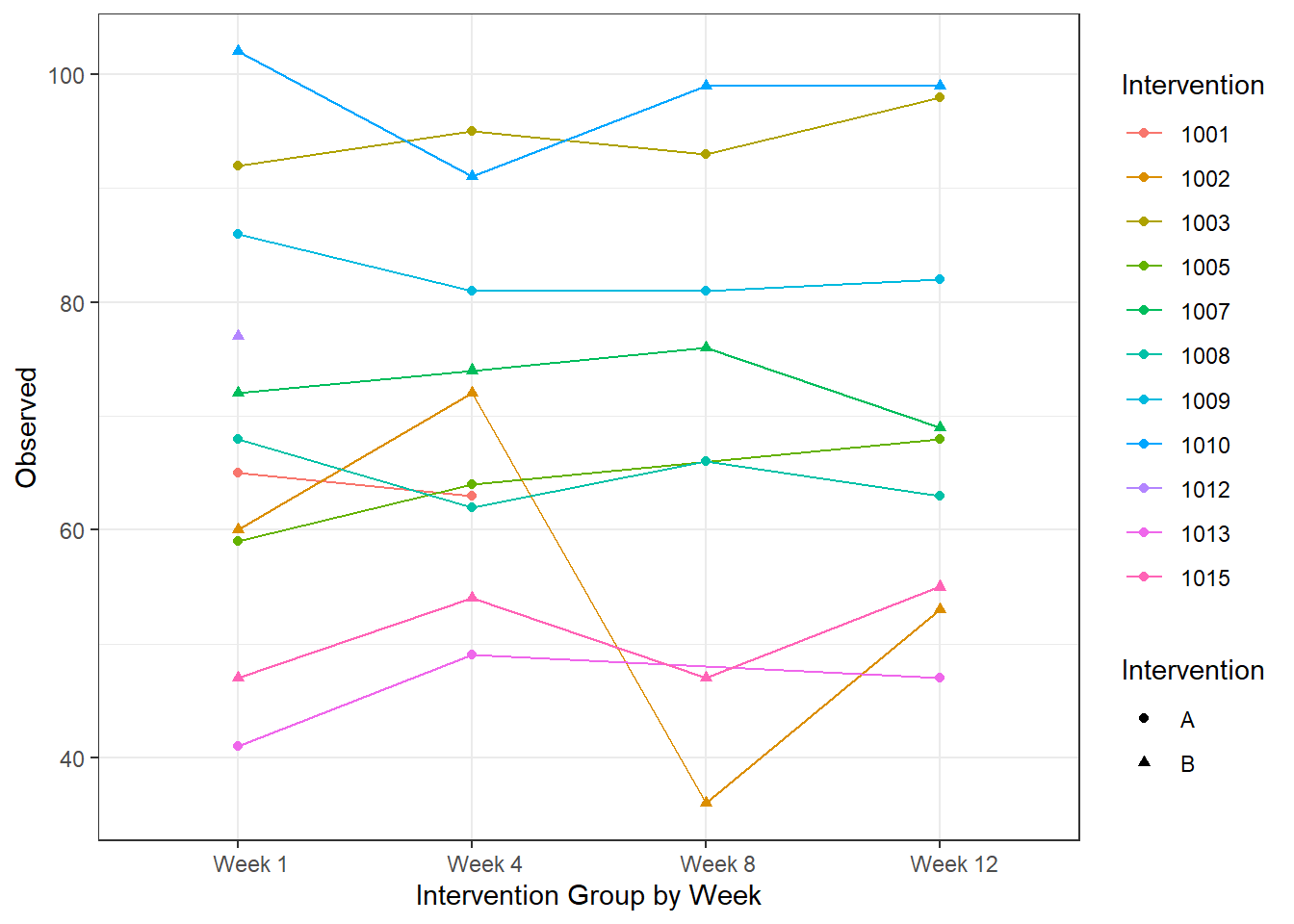
Shannon Index
ggplot(plot_data, aes(x=Intervention, y=Shannon,
                      group=Intervention,
                      color=Intervention, shape=Intervention))+
  geom_boxplot(outlier.alpha = 0)+
  geom_point(position="jitter")+
  facet_grid(.~Week)+
  labs(x="Intervention Group by Week")+
  guides(colour= guide_legend(title = "Intervention"))+
  theme(axis.text.x = element_text(angle = 0, hjust=0.33))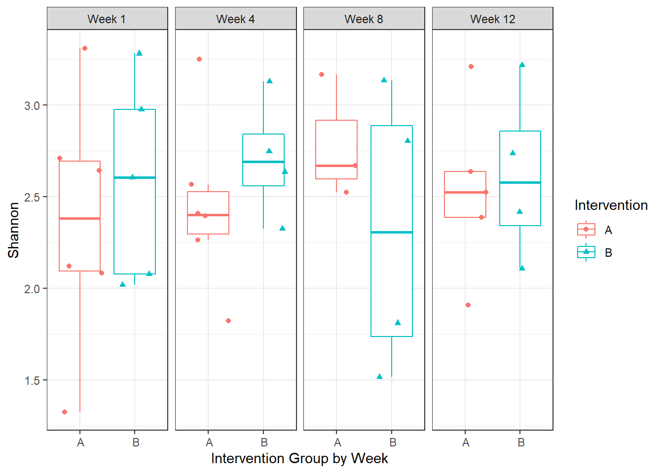
Simpson
ggplot(plot_data, aes(x=Intervention, y=Simpson,
                      group=Intervention,
                      color=Intervention, shape=Intervention))+
  geom_boxplot(outlier.alpha = 0)+
  geom_point(position="jitter")+
  facet_grid(.~Week)+
  labs(x="Intervention Group by Week")+
  guides(colour= guide_legend(title = "Intervention"))+
  theme(axis.text.x = element_text(angle = 0, hjust=0.33))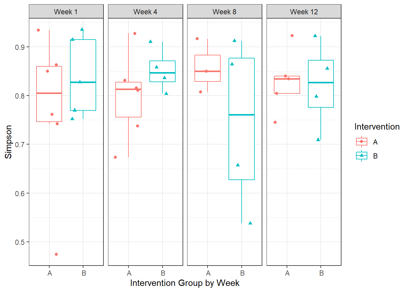
sessionInfo()R version 3.6.3 (2020-02-29)
Platform: x86_64-w64-mingw32/x64 (64-bit)
Running under: Windows 10 x64 (build 18362)
Matrix products: default
locale:
[1] LC_COLLATE=English_United States.1252
[2] LC_CTYPE=English_United States.1252
[3] LC_MONETARY=English_United States.1252
[4] LC_NUMERIC=C
[5] LC_TIME=English_United States.1252
attached base packages:
[1] stats graphics grDevices utils datasets methods base
other attached packages:
[1] cowplot_1.0.0 microbiome_1.8.0 car_3.0-8 carData_3.0-4
[5] gvlma_1.0.0.3 patchwork_1.0.0 viridis_0.5.1 viridisLite_0.3.0
[9] gridExtra_2.3 xtable_1.8-4 kableExtra_1.1.0 plyr_1.8.6
[13] data.table_1.12.8 readxl_1.3.1 forcats_0.5.0 stringr_1.4.0
[17] dplyr_0.8.5 purrr_0.3.4 readr_1.3.1 tidyr_1.1.0
[21] tibble_3.0.1 ggplot2_3.3.0 tidyverse_1.3.0 lmerTest_3.1-2
[25] lme4_1.1-23 Matrix_1.2-18 vegan_2.5-6 lattice_0.20-38
[29] permute_0.9-5 phyloseq_1.30.0
loaded via a namespace (and not attached):
[1] Rtsne_0.15 minqa_1.2.4 colorspace_1.4-1
[4] rio_0.5.16 ellipsis_0.3.1 rprojroot_1.3-2
[7] XVector_0.26.0 fs_1.4.1 rstudioapi_0.11
[10] farver_2.0.3 fansi_0.4.1 lubridate_1.7.8
[13] xml2_1.3.2 codetools_0.2-16 splines_3.6.3
[16] knitr_1.28 ade4_1.7-15 jsonlite_1.6.1
[19] workflowr_1.6.2 nloptr_1.2.2.1 broom_0.5.6
[22] cluster_2.1.0 dbplyr_1.4.4 BiocManager_1.30.10
[25] compiler_3.6.3 httr_1.4.1 backports_1.1.7
[28] assertthat_0.2.1 cli_2.0.2 later_1.0.0
[31] htmltools_0.4.0 tools_3.6.3 igraph_1.2.5
[34] gtable_0.3.0 glue_1.4.1 reshape2_1.4.4
[37] Rcpp_1.0.4.6 Biobase_2.46.0 cellranger_1.1.0
[40] vctrs_0.3.0 Biostrings_2.54.0 multtest_2.42.0
[43] ape_5.3 nlme_3.1-144 iterators_1.0.12
[46] xfun_0.14 openxlsx_4.1.5 rvest_0.3.5
[49] lifecycle_0.2.0 statmod_1.4.34 zlibbioc_1.32.0
[52] MASS_7.3-51.5 scales_1.1.1 hms_0.5.3
[55] promises_1.1.0 parallel_3.6.3 biomformat_1.14.0
[58] rhdf5_2.30.1 curl_4.3 yaml_2.2.1
[61] stringi_1.4.6 S4Vectors_0.24.4 foreach_1.5.0
[64] BiocGenerics_0.32.0 zip_2.0.4 boot_1.3-24
[67] rlang_0.4.6 pkgconfig_2.0.3 evaluate_0.14
[70] Rhdf5lib_1.8.0 labeling_0.3 tidyselect_1.1.0
[73] magrittr_1.5 R6_2.4.1 IRanges_2.20.2
[76] generics_0.0.2 DBI_1.1.0 foreign_0.8-75
[79] pillar_1.4.4 haven_2.3.0 whisker_0.4
[82] withr_2.2.0 mgcv_1.8-31 abind_1.4-5
[85] survival_3.1-8 modelr_0.1.8 crayon_1.3.4
[88] rmarkdown_2.1 grid_3.6.3 blob_1.2.1
[91] git2r_0.27.1 reprex_0.3.0 digest_0.6.25
[94] webshot_0.5.2 httpuv_1.5.2 numDeriv_2016.8-1.1
[97] stats4_3.6.3 munsell_0.5.0