Last updated: 2020-06-30

Checks: 6 1

Knit directory: Fiber_Intervention_Study/

This reproducible R Markdown analysis was created with workflowr (version 1.6.2). The Checks tab describes the reproducibility checks that were applied when the results were created. The Past versions tab lists the development history.

R Markdown file: uncommitted changes

The R Markdown file has unstaged changes. To know which version of the R Markdown file created these results, you’ll want to first commit it to the Git repo. If you’re still working on the analysis, you can ignore this warning. When you’re finished, you can run wflow_publish to commit the R Markdown file and build the HTML.

Environment: empty

Great job! The global environment was empty. Objects defined in the global environment can affect the analysis in your R Markdown file in unknown ways. For reproduciblity it’s best to always run the code in an empty environment.

Seed: set.seed(20191210)

The command set.seed(20191210) was run prior to running the code in the R Markdown file. Setting a seed ensures that any results that rely on randomness, e.g. subsampling or permutations, are reproducible.

Session information: recorded

Great job! Recording the operating system, R version, and package versions is critical for reproducibility.

Cache: none

Nice! There were no cached chunks for this analysis, so you can be confident that you successfully produced the results during this run.

File paths: relative

Great job! Using relative paths to the files within your workflowr project makes it easier to run your code on other machines.

Repository version: d377778

Great! You are using Git for version control. Tracking code development and connecting the code version to the results is critical for reproducibility.

The results in this page were generated with repository version d377778. See the Past versions tab to see a history of the changes made to the R Markdown and HTML files.

Note that you need to be careful to ensure that all relevant files for the analysis have been committed to Git prior to generating the results (you can use wflow_publish or wflow_git_commit). workflowr only checks the R Markdown file, but you know if there are other scripts or data files that it depends on. Below is the status of the Git repository when the results were generated:


Ignored files:
    Ignored:    .Rhistory
    Ignored:    .Rproj.user/
    Ignored:    code/.Rhistory
    Ignored:    reference-papers/Dietary_Variables.xlsx
    Ignored:    reference-papers/Johnson_2019.pdf
    Ignored:    renv/library/
    Ignored:    renv/staging/

Untracked files:
    Untracked:  analysis/hei_data_doublecheck.Rmd
    Untracked:  fig/figures-2020-06-21.zip
    Untracked:  fig/figures-2020-06-21/
    Untracked:  fig/figures-2020-06-23.zip
    Untracked:  fig/figures-2020-06-23/
    Untracked:  manuscript/Figures_2020_06_26.pdf
    Untracked:  manuscript/Manuscript Draft 2020-06-26[2].docx
    Untracked:  manuscript/Manuscript Draft 2020-06-28-NP.docx

Unstaged changes:
    Modified:   analysis/analysis_anthropometric.Rmd
    Deleted:    fig/figure1_alpha_diversity.pdf
    Deleted:    fig/figure1_legend.pdf
    Deleted:    fig/figure2_individual_beta_diversity_over_study.pdf
    Deleted:    fig/figure3_PCoA_analysis_results_beta_diversity_between_groups.pdf
    Deleted:    fig/figure3_legend.pdf
    Deleted:    fig/figure4_final_microbiome_diet_variables_over_time.pdf
    Deleted:    fig/figure4_legend.pdf
    Deleted:    fig/figure5_glmm_genus.pdf
    Deleted:    fig/figure5_glmm_phylum.pdf
    Deleted:    fig/figure6_change_in_BMI.pdf
    Modified:   fig/figures-2020-06-17.zip
    Modified:   tab/results_glmm_microbiome_genus.csv
    Modified:   tab/results_glmm_microbiome_phylum.csv

Note that any generated files, e.g. HTML, png, CSS, etc., are not included in this status report because it is ok for generated content to have uncommitted changes.

These are the previous versions of the repository in which changes were made to the R Markdown (analysis/analysis_anthropometric.Rmd) and HTML (docs/analysis_anthropometric.html) files. If you’ve configured a remote Git repository (see ?wflow_git_remote), click on the hyperlinks in the table below to view the files as they were in that past version.

File	Version	Author	Date	Message
html	9da43aa	noah-padgett	2020-06-08	Build site.
Rmd	94015da	noah-padgett	2020-06-08	revised figures
html	94015da	noah-padgett	2020-06-08	revised figures
html	0733fe5	noah-padgett	2020-05-21	Build site.
Rmd	d576bdd	noah-padgett	2020-05-21	tables outputted
html	d576bdd	noah-padgett	2020-05-21	tables outputted
Rmd	ef7cab9	noah-padgett	2020-05-14	blood measure analyses
Rmd	774a55f	noah-padgett	2020-04-16	updated beta diversity and permanova
html	774a55f	noah-padgett	2020-04-16	updated beta diversity and permanova

Overview of aims

What is the effect of Prebiotin vs placebo on anthropometrics (controlling for diet, age, ethnicity, stress?) Did the intervention mitigate excess weight gain?

BMI
Lean Body Mass
Visceral Fat Level
Weight

Therefore, data are analyzed at the last timepoint observed for each participant (week 12). If a participant is missing an outcome at week 12, the last observed score will be carried forward.

Analyses

What is the effect of Prebiotin vs. placebo on …

mydata <- microbiome_data$meta.dat
mydata <- arrange(mydata, desc(Week))
mydata <- distinct(mydata, SubjectID, .keep_all = T)
varNames <- c("SubjectID", "Week", "Age", "Ethnicity",
              "Gender", "Intervention", 
              "Height_cm", "Weight_pre", "Weight_post", 
              "LBM_pre", "LBM_post", "Visceral_Fat_Level_pre",
              "Visceral_Fat_Level_post", "Stress.Scale")
mydata <- mydata[, varNames]

mydata<- mydata %>%
  mutate(Weight_diff = Weight_pre - Weight_post,
         BMI_pre = Weight_pre/((Height_cm/100)**2),
         BMI_post = Weight_post/((Height_cm/100)**2),
         BMI_diff = BMI_pre - BMI_post,
         VFL_pre = Visceral_Fat_Level_pre,
         VFL_post = Visceral_Fat_Level_post,
         VFL_diff = VFL_pre - VFL_post,
         LBM_diff = LBM_pre - LBM_post,
         intB = ifelse(Intervention=="B", 1,0),
         c.age = Age - mean(Age),
         c.stress = Stress.Scale - mean(Stress.Scale),
         female = ifelse(Gender == "F", 1, 0),
         hispanic = ifelse(Ethnicity %in% c("White", "Asian", "Native America"), 1, 0))

plot.data <- mydata[,c(varNames[c(1:6,14,7:11)],  "Weight_diff", "BMI_pre", "BMI_post", "BMI_diff", "VFL_pre", "VFL_post", "VFL_diff", "LBM_diff")]
plot.data <- plot.data %>%
  pivot_longer(cols=c("Weight_pre", "Weight_post", "Weight_diff", "LBM_pre","LBM_post", "LBM_diff","BMI_pre", "BMI_post", "BMI_diff", "VFL_pre",  "VFL_post", "VFL_diff"),
               names_to = "Variable",
               values_to = "value")

Summary of these data is below

varNames <- c("intB", "female", "hispanic", "Age", "Stress.Scale",
              "Weight_pre", "Weight_post", "Weight_diff",
              "BMI_pre", "BMI_post", "BMI_diff",
              "LBM_pre", "LBM_post", "LBM_diff",
              "VFL_pre", "VFL_post", "VFL_diff")
sum.dat <- mydata[,varNames] %>%
  summarise_all(list(Mean=mean, SD=sd,
                     min=min, Median=median, Max=max))
sum.dat <- data.frame(matrix(unlist(sum.dat), ncol=5))
colnames(sum.dat) <- c("Mean", "SD", "Min", "Median", "Max")
rownames(sum.dat) <- varNames

kable(sum.dat, format="html", digits=3)%>%
  kable_styling(full_width = T)

	Mean	SD	Min	Median	Max
intB	0.455	0.522	0.000	0.000	1.000
female	0.636	0.505	0.000	1.000	1.000
hispanic	0.636	0.505	0.000	1.000	1.000
Age	27.818	2.040	26.000	27.000	32.000
Stress.Scale	12.818	4.535	7.000	13.000	21.000
Weight_pre	71.200	10.730	53.100	67.900	86.700
Weight_post	71.218	11.276	51.900	67.900	89.200
Weight_diff	-0.018	1.827	-4.300	0.200	1.800
BMI_pre	26.394	2.689	21.406	26.322	29.976
BMI_post	26.401	2.982	20.922	25.697	30.154
BMI_diff	-0.007	0.643	-1.442	0.075	0.625
LBM_pre	27.318	5.524	21.500	26.600	39.400
LBM_post	27.445	5.261	21.500	26.000	39.000
LBM_diff	-0.127	0.771	-1.900	0.000	0.600
VFL_pre	9.455	3.643	5.000	9.000	17.000
VFL_post	9.273	3.875	4.000	8.000	17.000
VFL_diff	0.182	0.982	-1.000	0.000	2.000

Summary of these data by Intervention Group

varNames <- c("Intervention",
              "female", "hispanic", "Age", "Stress.Scale",
              "Weight_pre", "Weight_post", "Weight_diff",
              "BMI_pre", "BMI_post", "BMI_diff",
              "LBM_pre", "LBM_post", "LBM_diff",
              "VFL_pre", "VFL_post", "VFL_diff")
sum.dat <- mydata[,varNames] %>%
  group_by(Intervention) %>%
  summarise_all(list(Mean=mean, SD=sd,
                     min=min, Median=median, Max=max))

a <- data.frame(matrix(unlist(sum.dat[1,-1]), ncol=5))
b <- data.frame(matrix(unlist(sum.dat[2,-1]), ncol=5))
a <- cbind(rep("A", 16), a); colnames(a) <- c("Intervention", "Mean", "SD", "Min", "Median", "Max")
b <- cbind(rep("B", 16), b); colnames(b) <- c("Intervention", "Mean", "SD", "Min", "Median", "Max")

sum.dat <- rbind(a,b)
sum.dat <- data.frame(Variable=rep(varNames[-1],2), sum.dat)
 
sum.dat <- arrange(sum.dat, Variable)
kable(sum.dat, format="html", digits=3)%>%
  kable_styling(full_width = T)

Variable	Intervention	Mean	SD	Min	Median	Max
Age	A	27.333	1.506	26.000	27.000	30.000
Age	B	28.400	2.608	26.000	28.000	32.000
BMI_diff	A	0.113	0.503	-0.524	0.279	0.577
BMI_diff	B	-0.150	0.818	-1.442	0.000	0.625
BMI_post	A	25.347	3.401	20.922	24.541	30.154
BMI_post	B	27.666	2.024	25.682	27.502	29.908
BMI_pre	A	25.460	3.127	21.406	24.787	29.630
BMI_pre	B	27.516	1.724	25.682	27.133	29.976
female	A	0.667	0.516	0.000	1.000	1.000
female	B	0.600	0.548	0.000	1.000	1.000
hispanic	A	0.500	0.548	0.000	0.500	1.000
hispanic	B	0.800	0.447	0.000	1.000	1.000
LBM_diff	A	-0.300	0.938	-1.900	0.000	0.600
LBM_diff	B	0.080	0.536	-0.600	0.100	0.600
LBM_post	A	27.167	6.447	21.500	24.800	39.000
LBM_post	B	27.780	4.121	22.100	27.400	32.600
LBM_pre	A	26.867	6.908	21.500	24.150	39.400
LBM_pre	B	27.860	3.996	22.200	27.100	32.000
Stress.Scale	A	10.667	3.204	7.000	11.000	15.000
Stress.Scale	B	15.400	4.827	8.000	15.000	21.000
VFL_diff	A	0.500	1.049	-1.000	0.500	2.000
VFL_diff	B	-0.200	0.837	-1.000	0.000	1.000
VFL_post	A	8.333	4.676	4.000	6.500	17.000
VFL_post	B	10.400	2.702	7.000	12.000	13.000
VFL_pre	A	8.833	4.309	5.000	8.000	17.000
VFL_pre	B	10.200	2.950	7.000	12.000	13.000
Weight_diff	A	0.367	1.363	-1.300	0.700	1.800
Weight_diff	B	-0.480	2.353	-4.300	0.000	1.600
Weight_post	A	68.600	12.146	51.900	68.700	84.900
Weight_post	B	74.360	10.527	65.800	67.900	89.200
Weight_pre	A	68.967	12.199	53.100	68.000	86.700
Weight_pre	B	73.880	9.238	66.200	67.900	84.900

Next, the aim is to more formally test for differences between intervention groups.

results.diff <- list()

BMI

# plot
p1 <- ggplot(filter(plot.data, Variable %like% "BMI"),
             aes(x=Variable, y=value))+
  geom_boxplot(outlier.shape = NA)+
  geom_jitter(width = 0.25)+
  scale_x_discrete(labels=c("BMI_pre"="Pre", "BMI_post"="Post"),
                   limits=c("BMI_pre", "BMI_post"))+
  labs(x=NULL, y="BMI", title="Pre and Post BMI")+
  theme(panel.grid = element_blank(),
        axis.text = element_text(size=10))
#p1

p2 <- ggplot(filter(plot.data, Variable %like% "BMI"),
             aes(x=Variable, y=value))+
  geom_boxplot(outlier.shape = NA)+
  geom_jitter(width = 0.25, size=2)+
  scale_x_discrete(labels=c("BMI_pre"="Pre", "BMI_post"="Post"),
                   limits=c("BMI_pre", "BMI_post"))+
  labs(x=NULL, y="BMI", title="Pre and Post BMI by Intervention Group")+
  facet_grid(.~Intervention, labeller = labeller(Intervention = c(A = "Group A", B = "Group B")))+
  theme(panel.grid = element_blank(),
        axis.text = element_text(size=10),
        strip.text = element_text(size=10))
#p2
p <- p1 + p2
p

Warning: Removed 11 rows containing missing values (stat_boxplot).

Warning: Removed 11 rows containing missing values (geom_point).

Warning: Removed 11 rows containing missing values (stat_boxplot).

Warning: Removed 11 rows containing missing values (geom_point).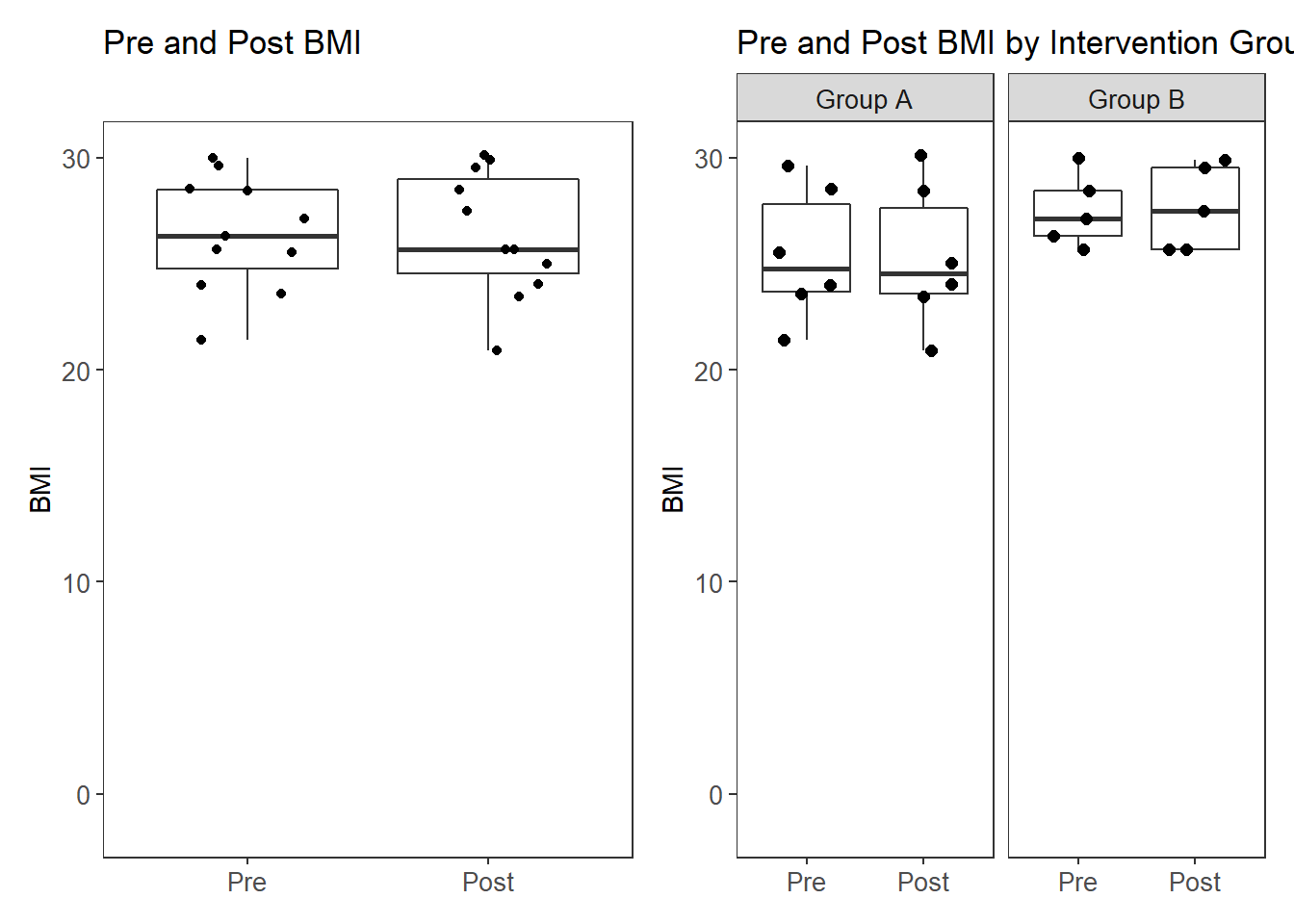

Pre BMI

This is simply to double check that no differences occured at baseline.

# Pre INtervention BMI - should beno difference
fit <- lm(BMI_pre ~ Intervention + c.age + hispanic + c.stress, mydata)
anova(fit)

Analysis of Variance Table

Response: BMI_pre
             Df Sum Sq Mean Sq F value Pr(>F)  
Intervention  1 11.525  11.525  2.7527 0.1482  
c.age         1  0.369   0.369  0.0881 0.7766  
hispanic      1 35.033  35.033  8.3673 0.0276 *
c.stress      1  0.273   0.273  0.0652 0.8069  
Residuals     6 25.121   4.187                 
---
Signif. codes:  0 '***' 0.001 '**' 0.01 '*' 0.05 '.' 0.1 ' ' 1

# diagnostic plots
layout(matrix(c(1,2,3,4),2,2)) # optional layout
plot(fit) # diagnostic plots

# normality again
shapiro.test(residuals(fit))


    Shapiro-Wilk normality test

data:  residuals(fit)
W = 0.9521, p-value = 0.6709

# independence
durbinWatsonTest(fit)

 lag Autocorrelation D-W Statistic p-value
   1      -0.3227466      2.393209    0.46
 Alternative hypothesis: rho != 0

layout(matrix(c(1),1,1))
acf(residuals(fit))

# nice wrapper function to generally test a lot of stuff
gvmodel <- gvlma(fit)
summary(gvmodel)


Call:
lm(formula = BMI_pre ~ Intervention + c.age + hispanic + c.stress, 
    data = mydata)

Residuals:
    Min      1Q  Median      3Q     Max 
-2.6671 -0.9978  0.2079  0.6727  2.6994 

Coefficients:
              Estimate Std. Error t value Pr(>|t|)    
(Intercept)   27.57014    1.14100  24.163  3.3e-07 ***
InterventionB  3.46721    2.12017   1.635   0.1531    
c.age         -0.35684    0.48903  -0.730   0.4931    
hispanic      -4.32429    1.65253  -2.617   0.0398 *  
c.stress       0.05628    0.22036   0.255   0.8069    
---
Signif. codes:  0 '***' 0.001 '**' 0.01 '*' 0.05 '.' 0.1 ' ' 1

Residual standard error: 2.046 on 6 degrees of freedom
Multiple R-squared:  0.6526,    Adjusted R-squared:  0.4211 
F-statistic: 2.818 on 4 and 6 DF,  p-value: 0.124


ASSESSMENT OF THE LINEAR MODEL ASSUMPTIONS
USING THE GLOBAL TEST ON 4 DEGREES-OF-FREEDOM:
Level of Significance =  0.05 

Call:
 gvlma(x = fit) 

                     Value p-value                   Decision
Global Stat        5.75961 0.21783    Assumptions acceptable.
Skewness           0.03115 0.85992    Assumptions acceptable.
Kurtosis           0.19354 0.65999    Assumptions acceptable.
Link Function      4.14455 0.04177 Assumptions NOT satisfied!
Heteroscedasticity 1.39037 0.23834    Assumptions acceptable.

No significant differences.

Post BMI

Test for significant differences after intervention

# Post INtervention BMI - should beno difference
# not controls
fit <- lm(BMI_post ~ Intervention, mydata)
anova(fit)

Analysis of Variance Table

Response: BMI_post
             Df Sum Sq Mean Sq F value Pr(>F)
Intervention  1 14.673 14.6730   1.779  0.215
Residuals     9 74.231  8.2479

summary(fit)


Call:
lm(formula = BMI_post ~ Intervention, data = mydata)

Residuals:
    Min      1Q  Median      3Q     Max 
-4.4244 -1.9352 -0.3242  2.0589  4.8071 

Coefficients:
              Estimate Std. Error t value Pr(>|t|)    
(Intercept)     25.347      1.172  21.618 4.57e-09 ***
InterventionB    2.320      1.739   1.334    0.215    
---
Signif. codes:  0 '***' 0.001 '**' 0.01 '*' 0.05 '.' 0.1 ' ' 1

Residual standard error: 2.872 on 9 degrees of freedom
Multiple R-squared:  0.165, Adjusted R-squared:  0.07227 
F-statistic: 1.779 on 1 and 9 DF,  p-value: 0.215

fit <- lm(BMI_post ~ Intervention + c.age + hispanic + c.stress,
          mydata)
anova(fit)

Analysis of Variance Table

Response: BMI_post
             Df Sum Sq Mean Sq F value  Pr(>F)  
Intervention  1 14.673  14.673  2.7695 0.14713  
c.age         1  0.602   0.602  0.1137 0.74747  
hispanic      1 41.131  41.131  7.7634 0.03173 *
c.stress      1  0.709   0.709  0.1339 0.72696  
Residuals     6 31.788   5.298                  
---
Signif. codes:  0 '***' 0.001 '**' 0.01 '*' 0.05 '.' 0.1 ' ' 1

summary(fit)


Call:
lm(formula = BMI_post ~ Intervention + c.age + hispanic + c.stress, 
    data = mydata)

Residuals:
    Min      1Q  Median      3Q     Max 
-2.6992 -1.1714  0.2195  1.1039  2.6958 

Coefficients:
              Estimate Std. Error t value Pr(>|t|)    
(Intercept)   27.56605    1.28351  21.477 6.65e-07 ***
InterventionB  3.88642    2.38498   1.630   0.1543    
c.age         -0.57580    0.55011  -1.047   0.3356    
hispanic      -4.60697    1.85893  -2.478   0.0479 *  
c.stress       0.09071    0.24789   0.366   0.7270    
---
Signif. codes:  0 '***' 0.001 '**' 0.01 '*' 0.05 '.' 0.1 ' ' 1

Residual standard error: 2.302 on 6 degrees of freedom
Multiple R-squared:  0.6424,    Adjusted R-squared:  0.4041 
F-statistic: 2.695 on 4 and 6 DF,  p-value: 0.1338

# diagnostic plots
layout(matrix(c(1,2,3,4),2,2)) # optional layout
plot(fit) # diagnostic plots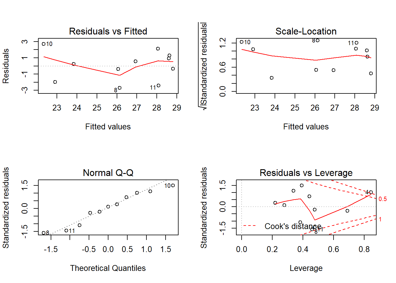

# normality again
shapiro.test(residuals(fit))


    Shapiro-Wilk normality test

data:  residuals(fit)
W = 0.95151, p-value = 0.6633

# independence
durbinWatsonTest(fit)

 lag Autocorrelation D-W Statistic p-value
   1      -0.3275118       2.33383   0.504
 Alternative hypothesis: rho != 0

layout(matrix(c(1),1,1))
acf(residuals(fit))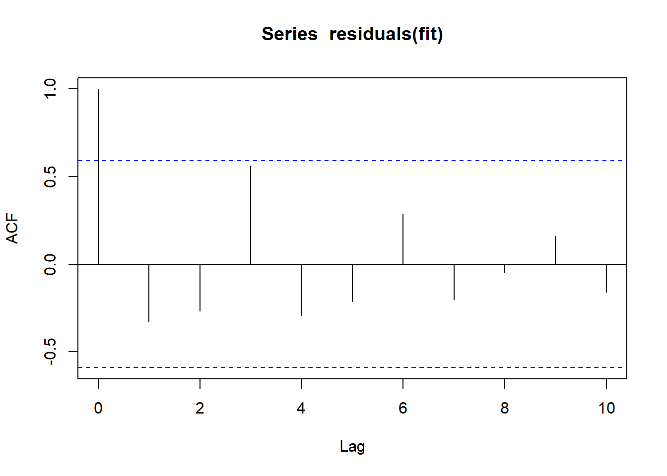

# nice wrapper function to generally test a lot of stuff
gvmodel <- gvlma(fit)
summary(gvmodel)


Call:
lm(formula = BMI_post ~ Intervention + c.age + hispanic + c.stress, 
    data = mydata)

Residuals:
    Min      1Q  Median      3Q     Max 
-2.6992 -1.1714  0.2195  1.1039  2.6958 

Coefficients:
              Estimate Std. Error t value Pr(>|t|)    
(Intercept)   27.56605    1.28351  21.477 6.65e-07 ***
InterventionB  3.88642    2.38498   1.630   0.1543    
c.age         -0.57580    0.55011  -1.047   0.3356    
hispanic      -4.60697    1.85893  -2.478   0.0479 *  
c.stress       0.09071    0.24789   0.366   0.7270    
---
Signif. codes:  0 '***' 0.001 '**' 0.01 '*' 0.05 '.' 0.1 ' ' 1

Residual standard error: 2.302 on 6 degrees of freedom
Multiple R-squared:  0.6424,    Adjusted R-squared:  0.4041 
F-statistic: 2.695 on 4 and 6 DF,  p-value: 0.1338


ASSESSMENT OF THE LINEAR MODEL ASSUMPTIONS
USING THE GLOBAL TEST ON 4 DEGREES-OF-FREEDOM:
Level of Significance =  0.05 

Call:
 gvlma(x = fit) 

                     Value p-value                Decision
Global Stat        4.82808 0.30540 Assumptions acceptable.
Skewness           0.05744 0.81058 Assumptions acceptable.
Kurtosis           0.51849 0.47148 Assumptions acceptable.
Link Function      3.11367 0.07764 Assumptions acceptable.
Heteroscedasticity 1.13847 0.28598 Assumptions acceptable.

No significant difference found.

Difference Scores of BMI

Test for significant differences after intervention

# Post INtervention BMI - should beno difference
# not controls
fit <- lm(BMI_diff ~ Intervention, mydata)
anova(fit)

Analysis of Variance Table

Response: BMI_diff
             Df Sum Sq Mean Sq F value Pr(>F)
Intervention  1 0.1898 0.18982  0.4332 0.5269
Residuals     9 3.9434 0.43815

summary(fit)


Call:
lm(formula = BMI_diff ~ Intervention, data = mydata)

Residuals:
    Min      1Q  Median      3Q     Max 
-1.2913 -0.3965  0.1505  0.4402  0.7753 

Coefficients:
              Estimate Std. Error t value Pr(>|t|)
(Intercept)     0.1133     0.2702   0.419    0.685
InterventionB  -0.2638     0.4008  -0.658    0.527

Residual standard error: 0.6619 on 9 degrees of freedom
Multiple R-squared:  0.04592,   Adjusted R-squared:  -0.06008 
F-statistic: 0.4332 on 1 and 9 DF,  p-value: 0.5269

fit <- lm(BMI_diff ~ Intervention + c.age + hispanic + c.stress,
          mydata)
anova(fit)

Analysis of Variance Table

Response: BMI_diff
             Df  Sum Sq Mean Sq F value  Pr(>F)  
Intervention  1 0.18982 0.18982  0.6768 0.44215  
c.age         1 1.91391 1.91391  6.8243 0.03999 *
hispanic      1 0.24454 0.24454  0.8719 0.38646  
c.stress      1 0.10221 0.10221  0.3644 0.56815  
Residuals     6 1.68273 0.28045                  
---
Signif. codes:  0 '***' 0.001 '**' 0.01 '*' 0.05 '.' 0.1 ' ' 1

summary(fit)


Call:
lm(formula = BMI_diff ~ Intervention + c.age + hispanic + c.stress, 
    data = mydata)

Residuals:
     Min       1Q   Median       3Q      Max 
-0.62947 -0.28789  0.00361  0.31689  0.60568 

Coefficients:
              Estimate Std. Error t value Pr(>|t|)
(Intercept)    0.00409    0.29531   0.014    0.989
InterventionB -0.41921    0.54873  -0.764    0.474
c.age          0.21896    0.12657   1.730    0.134
hispanic       0.28268    0.42770   0.661    0.533
c.stress      -0.03443    0.05703  -0.604    0.568

Residual standard error: 0.5296 on 6 degrees of freedom
Multiple R-squared:  0.5929,    Adjusted R-squared:  0.3215 
F-statistic: 2.184 on 4 and 6 DF,  p-value: 0.1875

results.diff[["BMI"]] <- summary(fit)[["coefficients"]]

# diagnostic plots
layout(matrix(c(1,2,3,4),2,2)) # optional layout
plot(fit) # diagnostic plots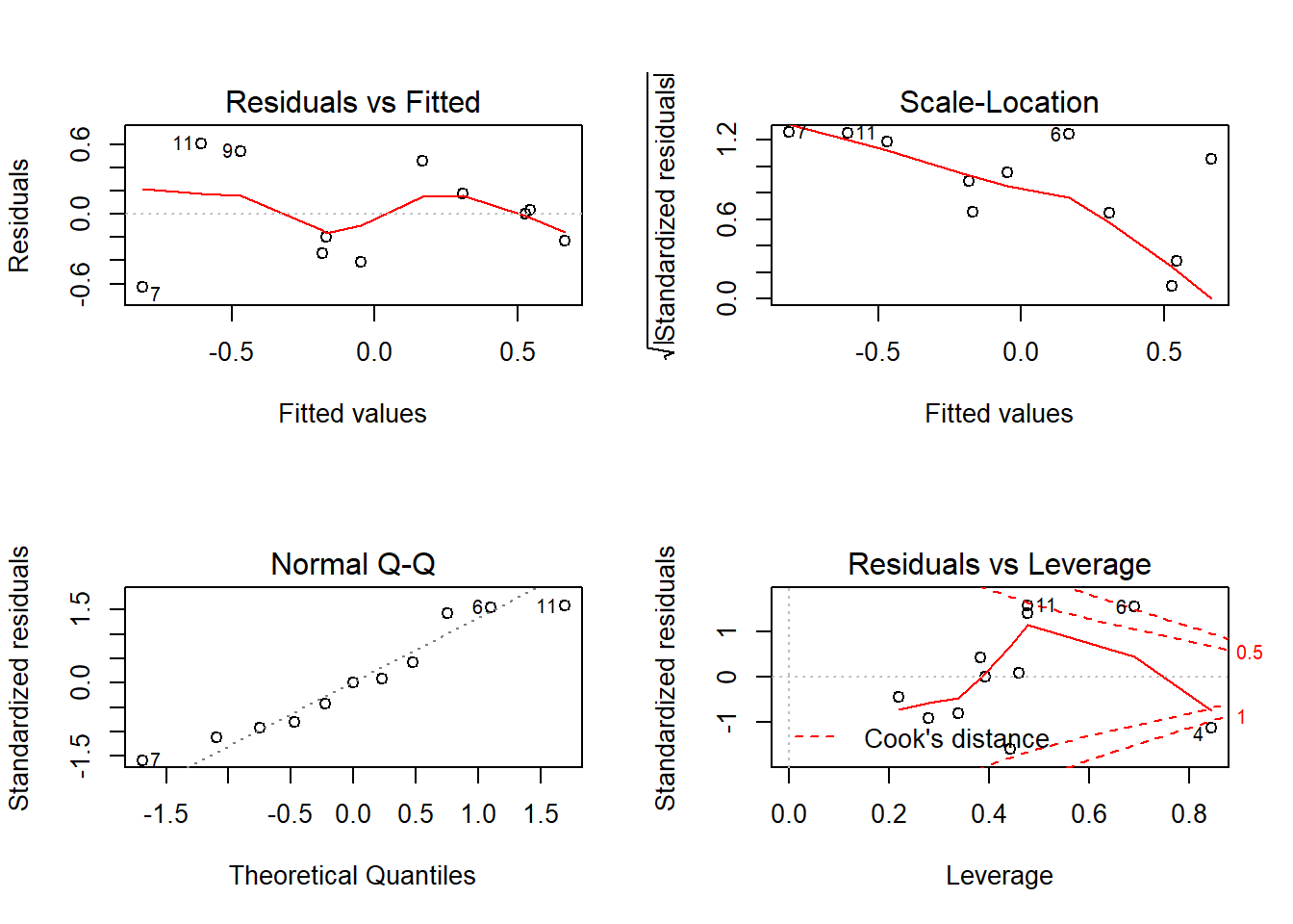

# normality again
shapiro.test(residuals(fit))


    Shapiro-Wilk normality test

data:  residuals(fit)
W = 0.95023, p-value = 0.6469

# independence
durbinWatsonTest(fit)

 lag Autocorrelation D-W Statistic p-value
   1      0.01418472      1.683813   0.658
 Alternative hypothesis: rho != 0

layout(matrix(c(1),1,1))
acf(residuals(fit))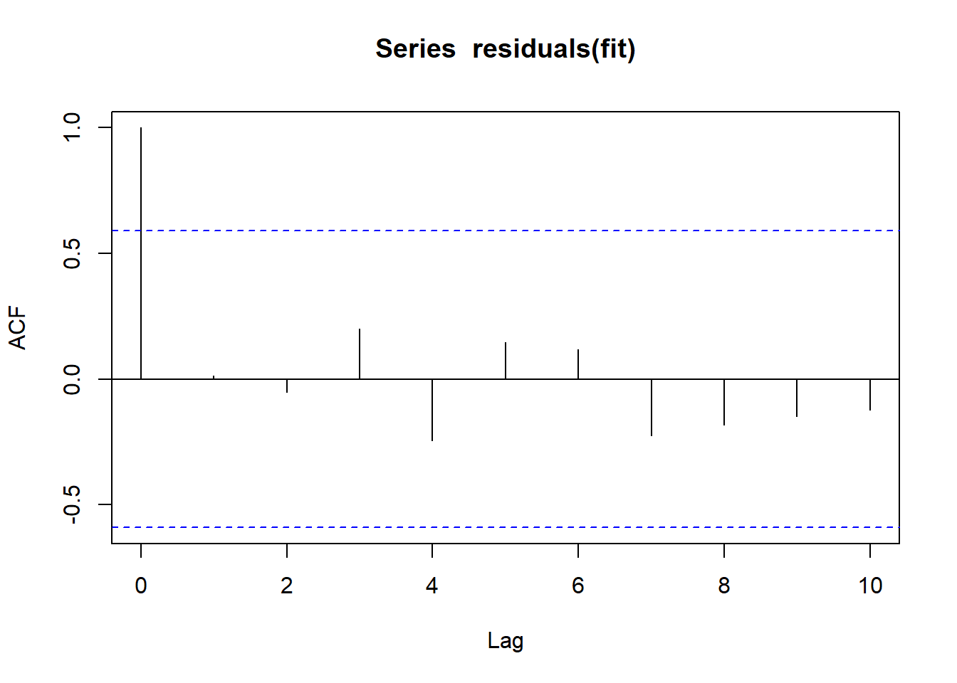

# nice wrapper function to generally test a lot of stuff
gvmodel <- gvlma(fit)
summary(gvmodel)


Call:
lm(formula = BMI_diff ~ Intervention + c.age + hispanic + c.stress, 
    data = mydata)

Residuals:
     Min       1Q   Median       3Q      Max 
-0.62947 -0.28789  0.00361  0.31689  0.60568 

Coefficients:
              Estimate Std. Error t value Pr(>|t|)
(Intercept)    0.00409    0.29531   0.014    0.989
InterventionB -0.41921    0.54873  -0.764    0.474
c.age          0.21896    0.12657   1.730    0.134
hispanic       0.28268    0.42770   0.661    0.533
c.stress      -0.03443    0.05703  -0.604    0.568

Residual standard error: 0.5296 on 6 degrees of freedom
Multiple R-squared:  0.5929,    Adjusted R-squared:  0.3215 
F-statistic: 2.184 on 4 and 6 DF,  p-value: 0.1875


ASSESSMENT OF THE LINEAR MODEL ASSUMPTIONS
USING THE GLOBAL TEST ON 4 DEGREES-OF-FREEDOM:
Level of Significance =  0.05 

Call:
 gvlma(x = fit) 

                     Value p-value                Decision
Global Stat        1.62530  0.8042 Assumptions acceptable.
Skewness           0.04558  0.8309 Assumptions acceptable.
Kurtosis           0.62676  0.4285 Assumptions acceptable.
Link Function      0.46154  0.4969 Assumptions acceptable.
Heteroscedasticity 0.49142  0.4833 Assumptions acceptable.

Therefore, we have evidence that BMI is not effected by Prebiotic vs. placebo.

Figure 6 changes in BMI

cols <- c("#00a2f2",  "#c91acb", "#7f5940", "#cc5200", "#00d957", "#40202d", "#e60099", "#006fa6", "#a6538a",  "#83008c", "#f29d3d","#a3d936", "#300059", "#566573", "#336655",  "#d9a3aa", "#400009", "#0020f2",  "#8091ff", "#fbffbf", "#00ffcc", "#8c4f46", "#354020", "#39c3e6", "#333a66", "#ff0000", "#6a8040",  "#730f00", "#0a4d00", "#ffe1bf", "#a3d9b1", "#003033", "#f29979", "#00b3a7", "#cbace6", "#bfd9ff", "#bf0000", "#293aa6", "#594943", "#e5c339", "#402910")


weight.dat <- filter(plot.data, Variable %in% c("BMI_pre", "BMI_post"))

weight.dat$time <- ifelse(weight.dat$Variable == "BMI_pre", "Pre", "Post")
weight.dat$time <- factor(weight.dat$time, levels=c("Pre", "Post"), ordered=T)

weight.dat$Group <- ifelse(weight.dat$Intervention == "A", "Placebo", "Intervention")
weight.dat$Group <- factor(weight.dat$Group, levels=c("Placebo", "Intervention"), ordered=T)

weight.dat$ID <- factor(weight.dat$SubjectID, levels=unique(weight.dat$SubjectID), labels=1:length(unique(weight.dat$SubjectID)))

p <- ggplot(weight.dat, aes(time, value, group=ID, color=ID, shape=Group)) +
  geom_line()+
  geom_point(size=3)+
  geom_hline(yintercept = 25, color="grey", linetype="dashed")+
  geom_hline(yintercept = 30, color="grey", linetype="dashed")+
  labs(y="BMI", x=NULL,
       title="Change in BMI from pre to post")+
  lims(y=c(20,32))+
  scale_color_manual(values=cols)+
  annotate("text", x=0.75, y=23, label="Normal")+
  annotate("text", x=0.75, y=27.5, label="Overweight")+
  annotate("text", x=0.75, y=31, label="Obese")+
  theme(panel.grid = element_blank(),
        axis.text.y = element_text(size=11),
        axis.text.x = element_text(size=11),
        axis.title.y = element_text(size=13),
        axis.title.x = element_blank())
p

Warning: Using shapes for an ordinal variable is not advised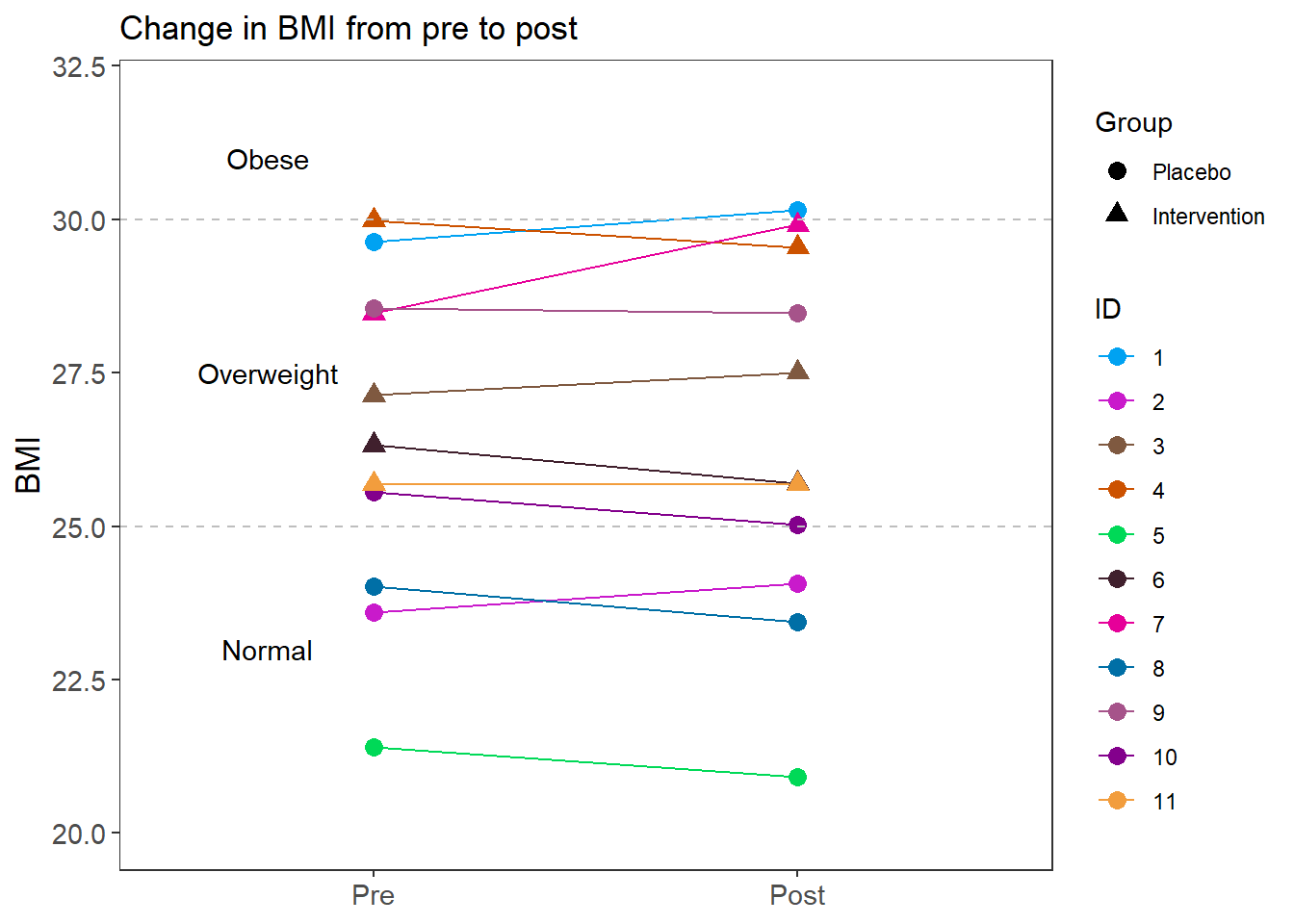

ggsave("fig/figure6.pdf", p, width=5,height=6, units="in")

Warning: Using shapes for an ordinal variable is not advised

#write.csv(weight.dat, paste0(w.d, "/tab/change_BMI.csv"))

Lean Body Mass (LBM)

# plot
p1 <- ggplot(filter(plot.data, Variable %like% "LBM"),
             aes(x=Variable, y=value))+
  geom_boxplot(outlier.shape = NA)+
  geom_jitter(width = 0.25, size=2)+
  scale_x_discrete(labels=c("LBM_pre"="Pre", "LBM_post"="Post"),
                   limits=c("LBM_pre", "LBM_post"))+
  labs(x=NULL, y="LBM", title="Pre and Post LBM")+
  theme(panel.grid = element_blank(),
        axis.text = element_text(size=10))
#p1

p2 <- ggplot(filter(plot.data, Variable %like% "LBM"),
             aes(x=Variable, y=value))+
  geom_boxplot(outlier.shape = NA)+
  geom_jitter(width = 0.25, size=2)+
  scale_x_discrete(labels=c("LBM_pre"="Pre", "LBM_post"="Post"),
                   limits=c("LBM_pre", "LBM_post"))+
  labs(x=NULL, y="LBM", title="Pre and Post LBM by Intervention Group")+
  facet_grid(.~Intervention, labeller = labeller(Intervention = c(A = "Group A", B = "Group B")))+
  theme(panel.grid = element_blank(),
        axis.text = element_text(size=10),
        strip.text = element_text(size=10))
#p2
p <- p1 + p2
p

Warning: Removed 11 rows containing missing values (stat_boxplot).

Warning: Removed 11 rows containing missing values (geom_point).

Warning: Removed 11 rows containing missing values (stat_boxplot).

Warning: Removed 11 rows containing missing values (geom_point).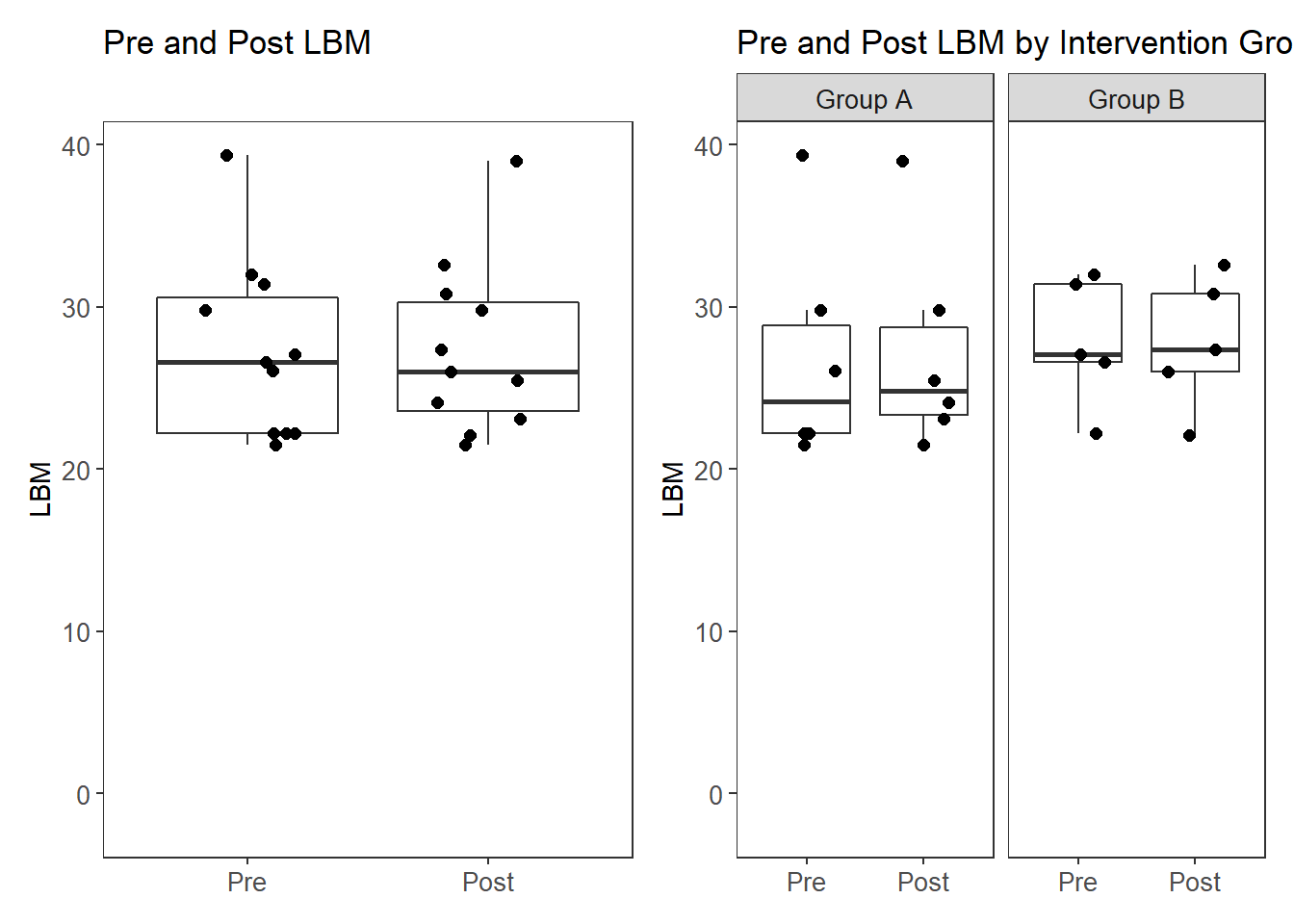

Pre LBM

This is simply to double check that no differences occured at baseline.

# Pre INtervention LBM - should beno difference
fit <- lm(LBM_pre ~ Intervention + c.age + hispanic + c.stress, mydata)
anova(fit)

Analysis of Variance Table

Response: LBM_pre
             Df  Sum Sq Mean Sq F value Pr(>F)
Intervention  1   2.691   2.691  0.0561 0.8206
c.age         1   2.124   2.124  0.0443 0.8402
hispanic      1   0.001   0.001  0.0000 0.9967
c.stress      1  12.775  12.775  0.2665 0.6241
Residuals     6 287.605  47.934

# diagnostic plots
layout(matrix(c(1,2,3,4),2,2)) # optional layout
plot(fit) # diagnostic plots

# normality again
shapiro.test(residuals(fit))


    Shapiro-Wilk normality test

data:  residuals(fit)
W = 0.9156, p-value = 0.2837

# independence
durbinWatsonTest(fit)

 lag Autocorrelation D-W Statistic p-value
   1       0.1254505      1.669594   0.562
 Alternative hypothesis: rho != 0

layout(matrix(c(1),1,1))
acf(residuals(fit))

# nice wrapper function to generally test a lot of stuff
gvmodel <- gvlma(fit)
summary(gvmodel)


Call:
lm(formula = LBM_pre ~ Intervention + c.age + hispanic + c.stress, 
    data = mydata)

Residuals:
    Min      1Q  Median      3Q     Max 
-6.3822 -4.1700 -0.8369  2.3452 11.8227 

Coefficients:
              Estimate Std. Error t value Pr(>|t|)    
(Intercept)    26.3882     3.8607   6.835 0.000482 ***
InterventionB   3.4391     7.1738   0.479 0.648631    
c.age          -0.3049     1.6547  -0.184 0.859875    
hispanic       -0.9950     5.5915  -0.178 0.864615    
c.stress       -0.3849     0.7456  -0.516 0.624142    
---
Signif. codes:  0 '***' 0.001 '**' 0.01 '*' 0.05 '.' 0.1 ' ' 1

Residual standard error: 6.923 on 6 degrees of freedom
Multiple R-squared:  0.05764,   Adjusted R-squared:  -0.5706 
F-statistic: 0.09175 on 4 and 6 DF,  p-value: 0.9816


ASSESSMENT OF THE LINEAR MODEL ASSUMPTIONS
USING THE GLOBAL TEST ON 4 DEGREES-OF-FREEDOM:
Level of Significance =  0.05 

Call:
 gvlma(x = fit) 

                      Value p-value                Decision
Global Stat        3.055492  0.5486 Assumptions acceptable.
Skewness           1.646157  0.1995 Assumptions acceptable.
Kurtosis           0.007273  0.9320 Assumptions acceptable.
Link Function      0.154379  0.6944 Assumptions acceptable.
Heteroscedasticity 1.247683  0.2640 Assumptions acceptable.

No significant differences.

Post LBM

Test for significant differences after intervention

# Post INtervention LBM - should beno difference
# not controls
fit <- lm(LBM_post ~ Intervention, mydata)
anova(fit)

Analysis of Variance Table

Response: LBM_post
             Df  Sum Sq Mean Sq F value Pr(>F)
Intervention  1   1.026  1.0259  0.0335 0.8589
Residuals     9 275.721 30.6357

summary(fit)


Call:
lm(formula = LBM_post ~ Intervention, data = mydata)

Residuals:
   Min     1Q Median     3Q    Max 
-5.680 -3.567 -1.667  2.827 11.833 

Coefficients:
              Estimate Std. Error t value Pr(>|t|)    
(Intercept)    27.1667     2.2596  12.023 7.58e-07 ***
InterventionB   0.6133     3.3516   0.183    0.859    
---
Signif. codes:  0 '***' 0.001 '**' 0.01 '*' 0.05 '.' 0.1 ' ' 1

Residual standard error: 5.535 on 9 degrees of freedom
Multiple R-squared:  0.003707,  Adjusted R-squared:  -0.107 
F-statistic: 0.03349 on 1 and 9 DF,  p-value: 0.8589

fit <- lm(LBM_post ~ Intervention + c.age + hispanic + c.stress,
          mydata)
anova(fit)

Analysis of Variance Table

Response: LBM_post
             Df  Sum Sq Mean Sq F value Pr(>F)
Intervention  1   1.026   1.026  0.0231 0.8841
c.age         1   0.094   0.094  0.0021 0.9647
hispanic      1   0.054   0.054  0.0012 0.9733
c.stress      1   9.506   9.506  0.2144 0.6597
Residuals     6 266.067  44.345

summary(fit)


Call:
lm(formula = LBM_post ~ Intervention + c.age + hispanic + c.stress, 
    data = mydata)

Residuals:
    Min      1Q  Median      3Q     Max 
-6.6654 -3.4551 -0.8474  2.3115 11.2320 

Coefficients:
              Estimate Std. Error t value Pr(>|t|)    
(Intercept)    26.6108     3.7133   7.166 0.000373 ***
InterventionB   2.8196     6.8999   0.409 0.696992    
c.age          -0.3974     1.5915  -0.250 0.811144    
hispanic       -0.7023     5.3780  -0.131 0.900371    
c.stress       -0.3320     0.7172  -0.463 0.659689    
---
Signif. codes:  0 '***' 0.001 '**' 0.01 '*' 0.05 '.' 0.1 ' ' 1

Residual standard error: 6.659 on 6 degrees of freedom
Multiple R-squared:  0.03859,   Adjusted R-squared:  -0.6023 
F-statistic: 0.06021 on 4 and 6 DF,  p-value: 0.9915

# diagnostic plots
layout(matrix(c(1,2,3,4),2,2)) # optional layout
plot(fit) # diagnostic plots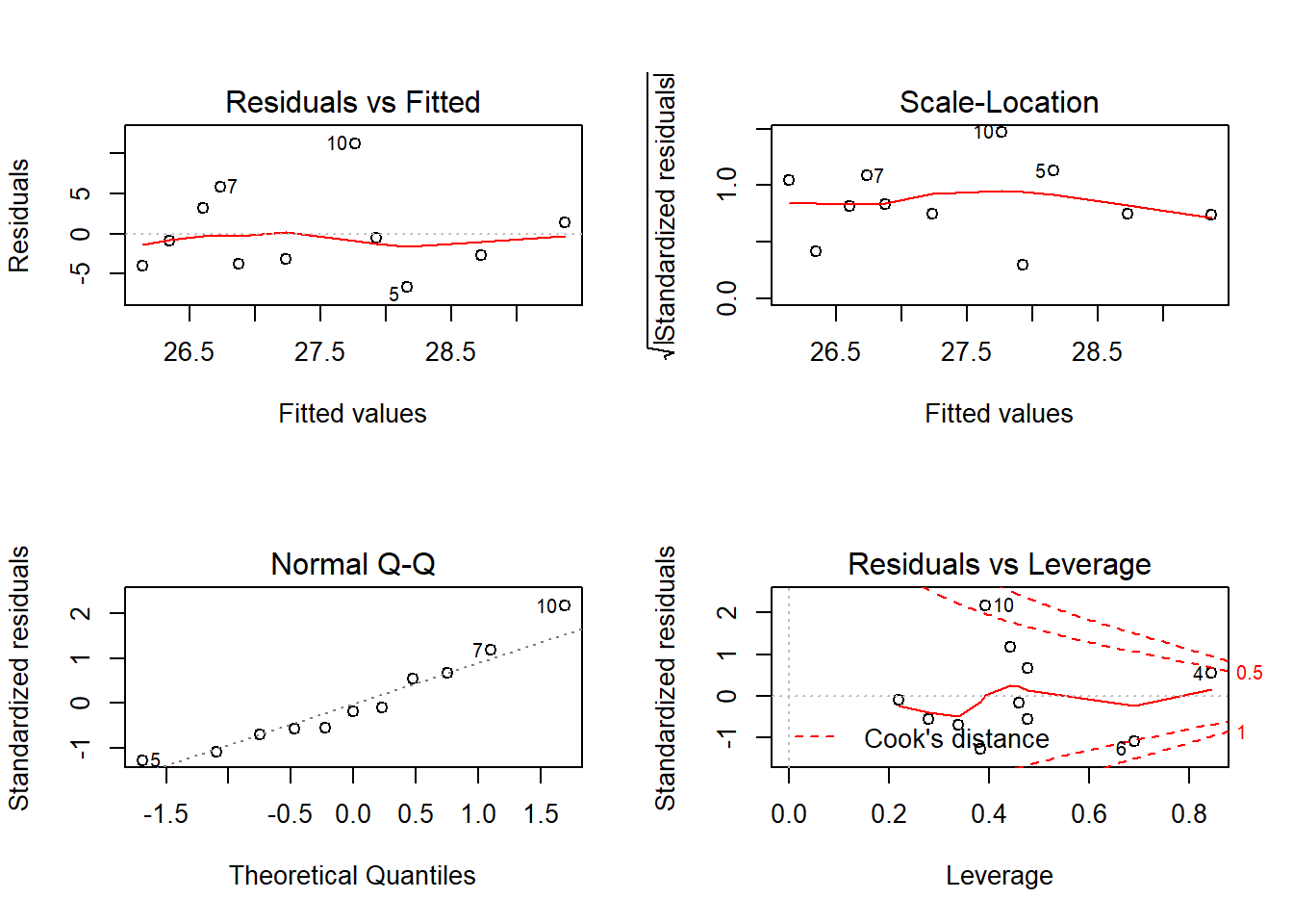

# normality again
shapiro.test(residuals(fit))


    Shapiro-Wilk normality test

data:  residuals(fit)
W = 0.92512, p-value = 0.3636

# independence
durbinWatsonTest(fit)

 lag Autocorrelation D-W Statistic p-value
   1      0.01493663      1.888619   0.888
 Alternative hypothesis: rho != 0

layout(matrix(c(1),1,1))
acf(residuals(fit))

# nice wrapper function to generally test a lot of stuff
gvmodel <- gvlma(fit)
summary(gvmodel)


Call:
lm(formula = LBM_post ~ Intervention + c.age + hispanic + c.stress, 
    data = mydata)

Residuals:
    Min      1Q  Median      3Q     Max 
-6.6654 -3.4551 -0.8474  2.3115 11.2320 

Coefficients:
              Estimate Std. Error t value Pr(>|t|)    
(Intercept)    26.6108     3.7133   7.166 0.000373 ***
InterventionB   2.8196     6.8999   0.409 0.696992    
c.age          -0.3974     1.5915  -0.250 0.811144    
hispanic       -0.7023     5.3780  -0.131 0.900371    
c.stress       -0.3320     0.7172  -0.463 0.659689    
---
Signif. codes:  0 '***' 0.001 '**' 0.01 '*' 0.05 '.' 0.1 ' ' 1

Residual standard error: 6.659 on 6 degrees of freedom
Multiple R-squared:  0.03859,   Adjusted R-squared:  -0.6023 
F-statistic: 0.06021 on 4 and 6 DF,  p-value: 0.9915


ASSESSMENT OF THE LINEAR MODEL ASSUMPTIONS
USING THE GLOBAL TEST ON 4 DEGREES-OF-FREEDOM:
Level of Significance =  0.05 

Call:
 gvlma(x = fit) 

                     Value p-value                Decision
Global Stat        3.68147  0.4508 Assumptions acceptable.
Skewness           1.50739  0.2195 Assumptions acceptable.
Kurtosis           0.00273  0.9583 Assumptions acceptable.
Link Function      0.61043  0.4346 Assumptions acceptable.
Heteroscedasticity 1.56092  0.2115 Assumptions acceptable.

Difference Scores of LBM

Test for significant differences after intervention

# Post INtervention LBM - should beno difference
# not controls
fit <- lm(LBM_diff ~ Intervention, mydata)
anova(fit)

Analysis of Variance Table

Response: LBM_diff
             Df Sum Sq Mean Sq F value Pr(>F)
Intervention  1 0.3938 0.39382  0.6389 0.4447
Residuals     9 5.5480 0.61644

summary(fit)


Call:
lm(formula = LBM_diff ~ Intervention, data = mydata)

Residuals:
   Min     1Q Median     3Q    Max 
 -1.60  -0.49   0.30   0.52   0.90 

Coefficients:
              Estimate Std. Error t value Pr(>|t|)
(Intercept)    -0.3000     0.3205  -0.936    0.374
InterventionB   0.3800     0.4754   0.799    0.445

Residual standard error: 0.7851 on 9 degrees of freedom
Multiple R-squared:  0.06628,   Adjusted R-squared:  -0.03747 
F-statistic: 0.6389 on 1 and 9 DF,  p-value: 0.4447

fit <- lm(LBM_diff ~ Intervention + c.age + hispanic + c.stress,
          mydata)
anova(fit)

Analysis of Variance Table

Response: LBM_diff
             Df Sum Sq Mean Sq F value Pr(>F)
Intervention  1 0.3938 0.39382  0.5993 0.4682
c.age         1 1.3230 1.32300  2.0133 0.2057
hispanic      1 0.0409 0.04091  0.0623 0.8113
c.stress      1 0.2412 0.24124  0.3671 0.5668
Residuals     6 3.9428 0.65714

summary(fit)


Call:
lm(formula = LBM_diff ~ Intervention + c.age + hispanic + c.stress, 
    data = mydata)

Residuals:
     Min       1Q   Median       3Q      Max 
-1.31265 -0.37213  0.06805  0.51538  0.77942 

Coefficients:
              Estimate Std. Error t value Pr(>|t|)
(Intercept)   -0.22258    0.45203  -0.492    0.640
InterventionB  0.61951    0.83995   0.738    0.489
c.age          0.09251    0.19374   0.478    0.650
hispanic      -0.29273    0.65469  -0.447    0.670
c.stress      -0.05289    0.08730  -0.606    0.567

Residual standard error: 0.8106 on 6 degrees of freedom
Multiple R-squared:  0.3364,    Adjusted R-squared:  -0.106 
F-statistic: 0.7605 on 4 and 6 DF,  p-value: 0.5871

results.diff[["LBM"]] <- summary(fit)[["coefficients"]]

# diagnostic plots
layout(matrix(c(1,2,3,4),2,2)) # optional layout
plot(fit) # diagnostic plots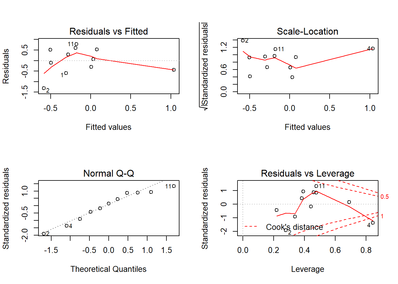

# normality again
shapiro.test(residuals(fit))


    Shapiro-Wilk normality test

data:  residuals(fit)
W = 0.93955, p-value = 0.5152

# independence
durbinWatsonTest(fit)

 lag Autocorrelation D-W Statistic p-value
   1       0.5506934     0.6556207   0.032
 Alternative hypothesis: rho != 0

layout(matrix(c(1),1,1))
acf(residuals(fit))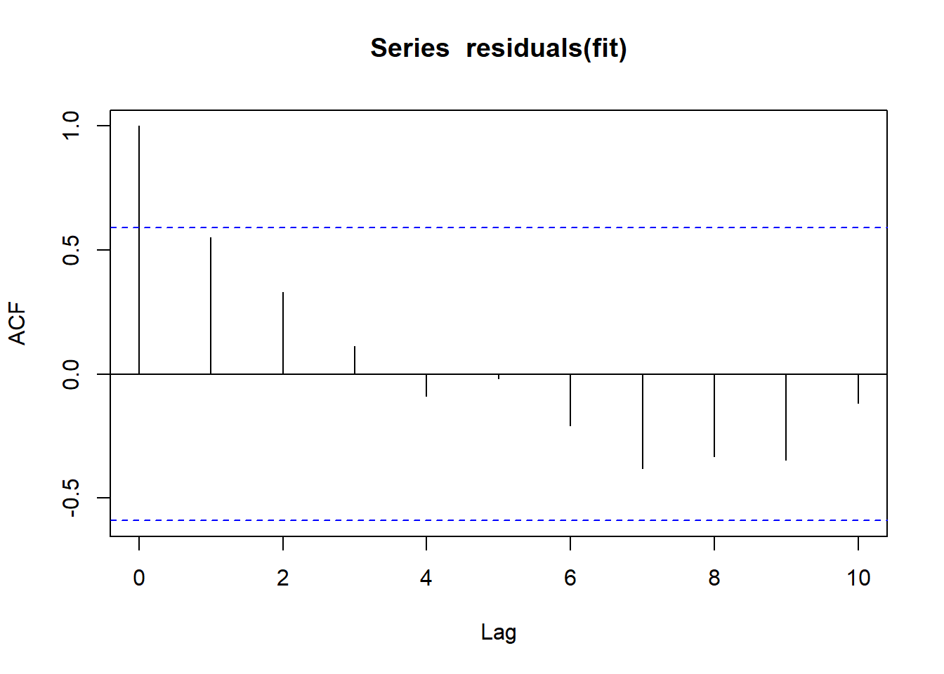

# nice wrapper function to generally test a lot of stuff
gvmodel <- gvlma(fit)
summary(gvmodel)


Call:
lm(formula = LBM_diff ~ Intervention + c.age + hispanic + c.stress, 
    data = mydata)

Residuals:
     Min       1Q   Median       3Q      Max 
-1.31265 -0.37213  0.06805  0.51538  0.77942 

Coefficients:
              Estimate Std. Error t value Pr(>|t|)
(Intercept)   -0.22258    0.45203  -0.492    0.640
InterventionB  0.61951    0.83995   0.738    0.489
c.age          0.09251    0.19374   0.478    0.650
hispanic      -0.29273    0.65469  -0.447    0.670
c.stress      -0.05289    0.08730  -0.606    0.567

Residual standard error: 0.8106 on 6 degrees of freedom
Multiple R-squared:  0.3364,    Adjusted R-squared:  -0.106 
F-statistic: 0.7605 on 4 and 6 DF,  p-value: 0.5871


ASSESSMENT OF THE LINEAR MODEL ASSUMPTIONS
USING THE GLOBAL TEST ON 4 DEGREES-OF-FREEDOM:
Level of Significance =  0.05 

Call:
 gvlma(x = fit) 

                     Value p-value                   Decision
Global Stat        5.24671 0.26291    Assumptions acceptable.
Skewness           0.84929 0.35675    Assumptions acceptable.
Kurtosis           0.04929 0.82430    Assumptions acceptable.
Link Function      3.88262 0.04879 Assumptions NOT satisfied!
Heteroscedasticity 0.46551 0.49506    Assumptions acceptable.

Therefore, we have evidence that LBM is not effected by Prebiotic vs. placebo.

Visceral Fat Level (VFL) Fat Mass

# plot
p1 <- ggplot(filter(plot.data, Variable %like% "VFL"),
             aes(x=Variable, y=value))+
  geom_boxplot(outlier.shape = NA)+
  geom_jitter(width = 0.25, size=2)+
  scale_x_discrete(labels=c("VFL_pre"="Pre", "VFL_post"="Post"),
                   limits=c("VFL_pre", "VFL_post"))+
  labs(x=NULL, y="VFL", title="Pre and Post VFL")+
  theme(panel.grid = element_blank(),
        axis.text = element_text(size=10))
#p1

p2 <- ggplot(filter(plot.data, Variable %like% "VFL"),
             aes(x=Variable, y=value))+
  geom_boxplot(outlier.shape = NA)+
  geom_jitter(width = 0.25, size=2)+
  scale_x_discrete(labels=c("VFL_pre"="Pre", "VFL_post"="Post"),
                   limits=c("VFL_pre", "VFL_post"))+
  labs(x=NULL, y="VFL", title="Pre and Post VFL by Intervention Group")+
  facet_grid(.~Intervention, labeller = labeller(Intervention = c(A = "Group A", B = "Group B")))+
  theme(panel.grid = element_blank(),
        axis.text = element_text(size=10),
        strip.text = element_text(size=10))
#p2
p <- p1 + p2
p

Warning: Removed 11 rows containing missing values (stat_boxplot).

Warning: Removed 11 rows containing missing values (geom_point).

Warning: Removed 11 rows containing missing values (stat_boxplot).

Warning: Removed 11 rows containing missing values (geom_point).

Pre VFL

This is simply to double check that no differences occured at baseline.

# Pre INtervention VFL - should beno difference
fit <- lm(VFL_pre ~ Intervention + c.age + hispanic + c.stress, mydata)
anova(fit)

Analysis of Variance Table

Response: VFL_pre
             Df Sum Sq Mean Sq F value Pr(>F)
Intervention  1  5.094  5.0939  0.3476 0.5770
c.age         1  0.632  0.6316  0.0431 0.8424
hispanic      1 25.724 25.7236  1.7551 0.2335
c.stress      1 13.340 13.3404  0.9102 0.3769
Residuals     6 87.938 14.6563

# diagnostic plots
layout(matrix(c(1,2,3,4),2,2)) # optional layout
plot(fit) # diagnostic plots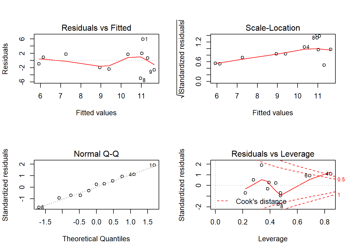

# normality again
shapiro.test(residuals(fit))


    Shapiro-Wilk normality test

data:  residuals(fit)
W = 0.96244, p-value = 0.8017

# independence
durbinWatsonTest(fit)

 lag Autocorrelation D-W Statistic p-value
   1      0.06653053      1.424408    0.31
 Alternative hypothesis: rho != 0

layout(matrix(c(1),1,1))
acf(residuals(fit))

# nice wrapper function to generally test a lot of stuff
gvmodel <- gvlma(fit)
summary(gvmodel)


Call:
lm(formula = VFL_pre ~ Intervention + c.age + hispanic + c.stress, 
    data = mydata)

Residuals:
    Min      1Q  Median      3Q     Max 
-4.9601 -2.1695  0.6951  1.6996  5.9273 

Coefficients:
              Estimate Std. Error t value Pr(>|t|)   
(Intercept)    11.1850     2.1348   5.239  0.00194 **
InterventionB   0.1030     3.9668   0.026  0.98013   
c.age           0.2247     0.9150   0.246  0.81417   
hispanic       -2.7929     3.0918  -0.903  0.40117   
c.stress        0.3933     0.4123   0.954  0.37690   
---
Signif. codes:  0 '***' 0.001 '**' 0.01 '*' 0.05 '.' 0.1 ' ' 1

Residual standard error: 3.828 on 6 degrees of freedom
Multiple R-squared:  0.3375,    Adjusted R-squared:  -0.1042 
F-statistic: 0.764 on 4 and 6 DF,  p-value: 0.5853


ASSESSMENT OF THE LINEAR MODEL ASSUMPTIONS
USING THE GLOBAL TEST ON 4 DEGREES-OF-FREEDOM:
Level of Significance =  0.05 

Call:
 gvlma(x = fit) 

                     Value p-value                Decision
Global Stat        1.23558  0.8722 Assumptions acceptable.
Skewness           0.12366  0.7251 Assumptions acceptable.
Kurtosis           0.01832  0.8923 Assumptions acceptable.
Link Function      0.08793  0.7668 Assumptions acceptable.
Heteroscedasticity 1.00567  0.3159 Assumptions acceptable.

No significant differences.

Post VFL

Test for significant differences after intervention

# Post INtervention VFL - should beno difference
# not controls
fit <- lm(VFL_post ~ Intervention, mydata)
anova(fit)

Analysis of Variance Table

Response: VFL_post
             Df  Sum Sq Mean Sq F value Pr(>F)
Intervention  1  11.648  11.649  0.7568 0.4069
Residuals     9 138.533  15.393

summary(fit)


Call:
lm(formula = VFL_post ~ Intervention, data = mydata)

Residuals:
   Min     1Q Median     3Q    Max 
-4.333 -2.367 -1.333  1.633  8.667 

Coefficients:
              Estimate Std. Error t value Pr(>|t|)    
(Intercept)      8.333      1.602   5.203 0.000562 ***
InterventionB    2.067      2.376   0.870 0.406947    
---
Signif. codes:  0 '***' 0.001 '**' 0.01 '*' 0.05 '.' 0.1 ' ' 1

Residual standard error: 3.923 on 9 degrees of freedom
Multiple R-squared:  0.07756,   Adjusted R-squared:  -0.02493 
F-statistic: 0.7568 on 1 and 9 DF,  p-value: 0.4069

fit <- lm(VFL_post ~ Intervention + c.age + hispanic + c.stress,
          mydata)
anova(fit)

Analysis of Variance Table

Response: VFL_post
             Df Sum Sq Mean Sq F value  Pr(>F)  
Intervention  1 11.648  11.648  0.9706 0.36258  
c.age         1  0.006   0.006  0.0005 0.98339  
hispanic      1 53.250  53.250  4.4369 0.07977 .
c.stress      1 13.269  13.269  1.1056 0.33353  
Residuals     6 72.009  12.002                  
---
Signif. codes:  0 '***' 0.001 '**' 0.01 '*' 0.05 '.' 0.1 ' ' 1

summary(fit)


Call:
lm(formula = VFL_post ~ Intervention + c.age + hispanic + c.stress, 
    data = mydata)

Residuals:
    Min      1Q  Median      3Q     Max 
-4.3890 -2.0123  0.6177  1.3834  5.4733 

Coefficients:
              Estimate Std. Error t value Pr(>|t|)   
(Intercept)    11.3591     1.9318   5.880  0.00107 **
InterventionB   1.6786     3.5896   0.468  0.65655   
c.age          -0.1177     0.8280  -0.142  0.89163   
hispanic       -4.4775     2.7978  -1.600  0.16064   
c.stress        0.3923     0.3731   1.051  0.33353   
---
Signif. codes:  0 '***' 0.001 '**' 0.01 '*' 0.05 '.' 0.1 ' ' 1

Residual standard error: 3.464 on 6 degrees of freedom
Multiple R-squared:  0.5205,    Adjusted R-squared:  0.2009 
F-statistic: 1.628 on 4 and 6 DF,  p-value: 0.2824

# diagnostic plots
layout(matrix(c(1,2,3,4),2,2)) # optional layout
plot(fit) # diagnostic plots

# normality again
shapiro.test(residuals(fit))


    Shapiro-Wilk normality test

data:  residuals(fit)
W = 0.95397, p-value = 0.695

# independence
durbinWatsonTest(fit)

 lag Autocorrelation D-W Statistic p-value
   1     -0.01794009       1.58296   0.452
 Alternative hypothesis: rho != 0

layout(matrix(c(1),1,1))
acf(residuals(fit))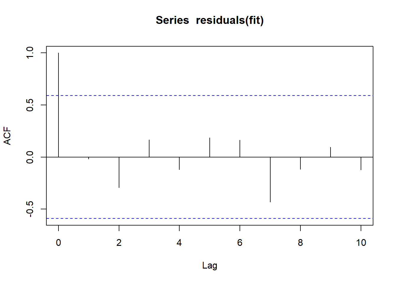

# nice wrapper function to generally test a lot of stuff
gvmodel <- gvlma(fit)
summary(gvmodel)


Call:
lm(formula = VFL_post ~ Intervention + c.age + hispanic + c.stress, 
    data = mydata)

Residuals:
    Min      1Q  Median      3Q     Max 
-4.3890 -2.0123  0.6177  1.3834  5.4733 

Coefficients:
              Estimate Std. Error t value Pr(>|t|)   
(Intercept)    11.3591     1.9318   5.880  0.00107 **
InterventionB   1.6786     3.5896   0.468  0.65655   
c.age          -0.1177     0.8280  -0.142  0.89163   
hispanic       -4.4775     2.7978  -1.600  0.16064   
c.stress        0.3923     0.3731   1.051  0.33353   
---
Signif. codes:  0 '***' 0.001 '**' 0.01 '*' 0.05 '.' 0.1 ' ' 1

Residual standard error: 3.464 on 6 degrees of freedom
Multiple R-squared:  0.5205,    Adjusted R-squared:  0.2009 
F-statistic: 1.628 on 4 and 6 DF,  p-value: 0.2824


ASSESSMENT OF THE LINEAR MODEL ASSUMPTIONS
USING THE GLOBAL TEST ON 4 DEGREES-OF-FREEDOM:
Level of Significance =  0.05 

Call:
 gvlma(x = fit) 

                      Value p-value                Decision
Global Stat        1.833660  0.7663 Assumptions acceptable.
Skewness           0.180994  0.6705 Assumptions acceptable.
Kurtosis           0.006109  0.9377 Assumptions acceptable.
Link Function      0.709705  0.3995 Assumptions acceptable.
Heteroscedasticity 0.936852  0.3331 Assumptions acceptable.

Difference Scores of VFL

Test for significant differences after intervention

# Post INtervention VFL - should beno difference
# not controls
fit <- lm(VFL_diff ~ Intervention, mydata)
anova(fit)

Analysis of Variance Table

Response: VFL_diff
             Df Sum Sq Mean Sq F value Pr(>F)
Intervention  1 1.3364 1.33636  1.4491 0.2594
Residuals     9 8.3000 0.92222

summary(fit)


Call:
lm(formula = VFL_diff ~ Intervention, data = mydata)

Residuals:
   Min     1Q Median     3Q    Max 
 -1.50  -0.65   0.20   0.50   1.50 

Coefficients:
              Estimate Std. Error t value Pr(>|t|)
(Intercept)     0.5000     0.3921   1.275    0.234
InterventionB  -0.7000     0.5815  -1.204    0.259

Residual standard error: 0.9603 on 9 degrees of freedom
Multiple R-squared:  0.1387,    Adjusted R-squared:  0.04298 
F-statistic: 1.449 on 1 and 9 DF,  p-value: 0.2594

fit <- lm(VFL_diff ~ Intervention + c.age + hispanic + c.stress,
          mydata)
anova(fit)

Analysis of Variance Table

Response: VFL_diff
             Df Sum Sq Mean Sq F value  Pr(>F)  
Intervention  1 1.3364  1.3364  3.0949 0.12903  
c.age         1 0.7567  0.7567  1.7525 0.23376  
hispanic      1 4.9523  4.9523 11.4690 0.01474 *
c.stress      1 0.0001  0.0001  0.0002 0.98860  
Residuals     6 2.5908  0.4318                  
---
Signif. codes:  0 '***' 0.001 '**' 0.01 '*' 0.05 '.' 0.1 ' ' 1

summary(fit)


Call:
lm(formula = VFL_diff ~ Intervention + c.age + hispanic + c.stress, 
    data = mydata)

Residuals:
    Min      1Q  Median      3Q     Max 
-0.5711 -0.3179 -0.2057  0.3177  1.1139 

Coefficients:
               Estimate Std. Error t value Pr(>|t|)  
(Intercept)   -0.174025   0.366424  -0.475   0.6516  
InterventionB -1.575594   0.680876  -2.314   0.0599 .
c.age          0.342395   0.157049   2.180   0.0720 .
hispanic       1.684606   0.530697   3.174   0.0192 *
c.stress       0.001054   0.070768   0.015   0.9886  
---
Signif. codes:  0 '***' 0.001 '**' 0.01 '*' 0.05 '.' 0.1 ' ' 1

Residual standard error: 0.6571 on 6 degrees of freedom
Multiple R-squared:  0.7311,    Adjusted R-squared:  0.5519 
F-statistic: 4.079 on 4 and 6 DF,  p-value: 0.06206

results.diff[["VFL"]] <- summary(fit)[["coefficients"]]

# diagnostic plots
layout(matrix(c(1,2,3,4),2,2)) # optional layout
plot(fit) # diagnostic plots

# normality again
shapiro.test(residuals(fit))


    Shapiro-Wilk normality test

data:  residuals(fit)
W = 0.90718, p-value = 0.2257

# independence
durbinWatsonTest(fit)

 lag Autocorrelation D-W Statistic p-value
   1       0.3316722       1.21887   0.204
 Alternative hypothesis: rho != 0

layout(matrix(c(1),1,1))
acf(residuals(fit))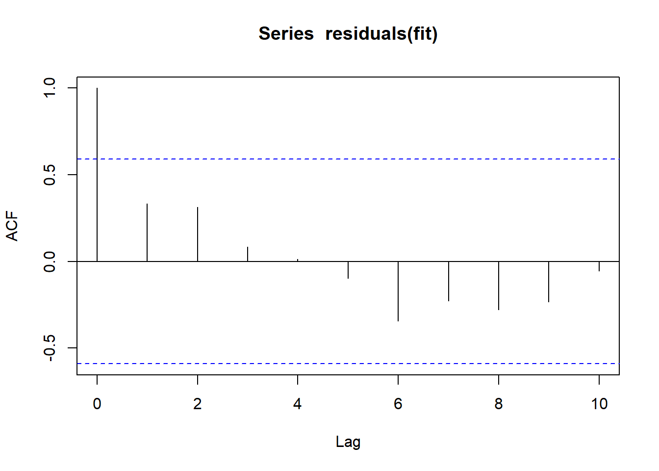

# nice wrapper function to generally test a lot of stuff
gvmodel <- gvlma(fit)
summary(gvmodel)


Call:
lm(formula = VFL_diff ~ Intervention + c.age + hispanic + c.stress, 
    data = mydata)

Residuals:
    Min      1Q  Median      3Q     Max 
-0.5711 -0.3179 -0.2057  0.3177  1.1139 

Coefficients:
               Estimate Std. Error t value Pr(>|t|)  
(Intercept)   -0.174025   0.366424  -0.475   0.6516  
InterventionB -1.575594   0.680876  -2.314   0.0599 .
c.age          0.342395   0.157049   2.180   0.0720 .
hispanic       1.684606   0.530697   3.174   0.0192 *
c.stress       0.001054   0.070768   0.015   0.9886  
---
Signif. codes:  0 '***' 0.001 '**' 0.01 '*' 0.05 '.' 0.1 ' ' 1

Residual standard error: 0.6571 on 6 degrees of freedom
Multiple R-squared:  0.7311,    Adjusted R-squared:  0.5519 
F-statistic: 4.079 on 4 and 6 DF,  p-value: 0.06206


ASSESSMENT OF THE LINEAR MODEL ASSUMPTIONS
USING THE GLOBAL TEST ON 4 DEGREES-OF-FREEDOM:
Level of Significance =  0.05 

Call:
 gvlma(x = fit) 

                       Value p-value                Decision
Global Stat        6.1228904 0.19016 Assumptions acceptable.
Skewness           1.3706785 0.24170 Assumptions acceptable.
Kurtosis           0.0000427 0.99479 Assumptions acceptable.
Link Function      3.6962650 0.05453 Assumptions acceptable.
Heteroscedasticity 1.0559042 0.30415 Assumptions acceptable.

Therefore, we have evidence that LBM is not effected by Prebiotic vs. placebo.

Weight (kg)

# plot
p1 <- ggplot(filter(plot.data, Variable %like% "Weight"),
             aes(x=Variable, y=value))+
  geom_boxplot(outlier.shape = NA)+
  geom_jitter(width = 0.25, size=2)+
  scale_x_discrete(labels=c("Weight_pre"="Pre", "Weight_post"="Post"),
                   limits=c("Weight_pre", "Weight_post"))+
  labs(x=NULL, y="Weight (kg)", title="Pre and Post Weight (kg)")+
  theme(panel.grid = element_blank(),
        axis.text = element_text(size=10))
#p1

p2 <- ggplot(filter(plot.data, Variable %like% "Weight"),
             aes(x=Variable, y=value))+
  geom_boxplot(outlier.shape = NA)+
  geom_jitter(width = 0.25, size=2)+
  scale_x_discrete(labels=c("Weight_pre"="Pre", "Weight_post"="Post"),
                   limits=c("Weight_pre", "Weight_post"))+
  labs(x=NULL, y="Weight (kg)", title="Pre and Post Weight (kg) by Intervention Group")+
  facet_grid(.~Intervention, labeller = labeller(Intervention = c(A = "Group A", B = "Group B")))+
  theme(panel.grid = element_blank(),
        axis.text = element_text(size=10),
        strip.text = element_text(size=10))
#p2
p <- p1 + p2
p

Warning: Removed 11 rows containing missing values (stat_boxplot).

Warning: Removed 11 rows containing missing values (geom_point).

Warning: Removed 11 rows containing missing values (stat_boxplot).

Warning: Removed 11 rows containing missing values (geom_point).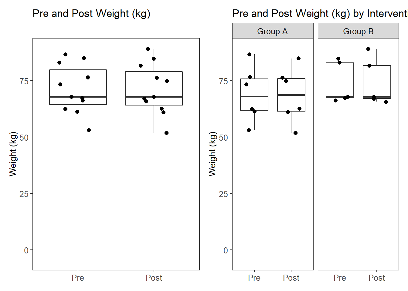

Pre Weight

This is simply to double check that no differences occured at baseline.

# Pre INtervention Weight - should beno difference
fit <- lm(Weight_pre ~ Intervention + c.age + hispanic + c.stress, mydata)
anova(fit)

Analysis of Variance Table

Response: Weight_pre
             Df Sum Sq Mean Sq F value Pr(>F)
Intervention  1  65.84  65.839  0.4038 0.5486
c.age         1   3.56   3.557  0.0218 0.8874
hispanic      1 102.90 102.900  0.6311 0.4572
c.stress      1   0.69   0.691  0.0042 0.9502
Residuals     6 978.31 163.052

# diagnostic plots
layout(matrix(c(1,2,3,4),2,2)) # optional layout
plot(fit) # diagnostic plots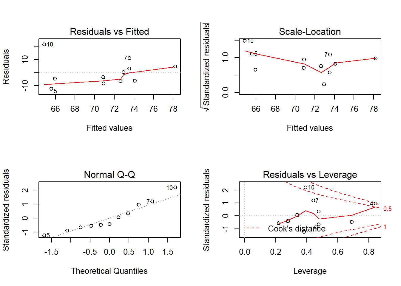

# normality again
shapiro.test(residuals(fit))


    Shapiro-Wilk normality test

data:  residuals(fit)
W = 0.92009, p-value = 0.3194

# independence
durbinWatsonTest(fit)

 lag Autocorrelation D-W Statistic p-value
   1       -0.254796       2.46993     0.4
 Alternative hypothesis: rho != 0

layout(matrix(c(1),1,1))
acf(residuals(fit))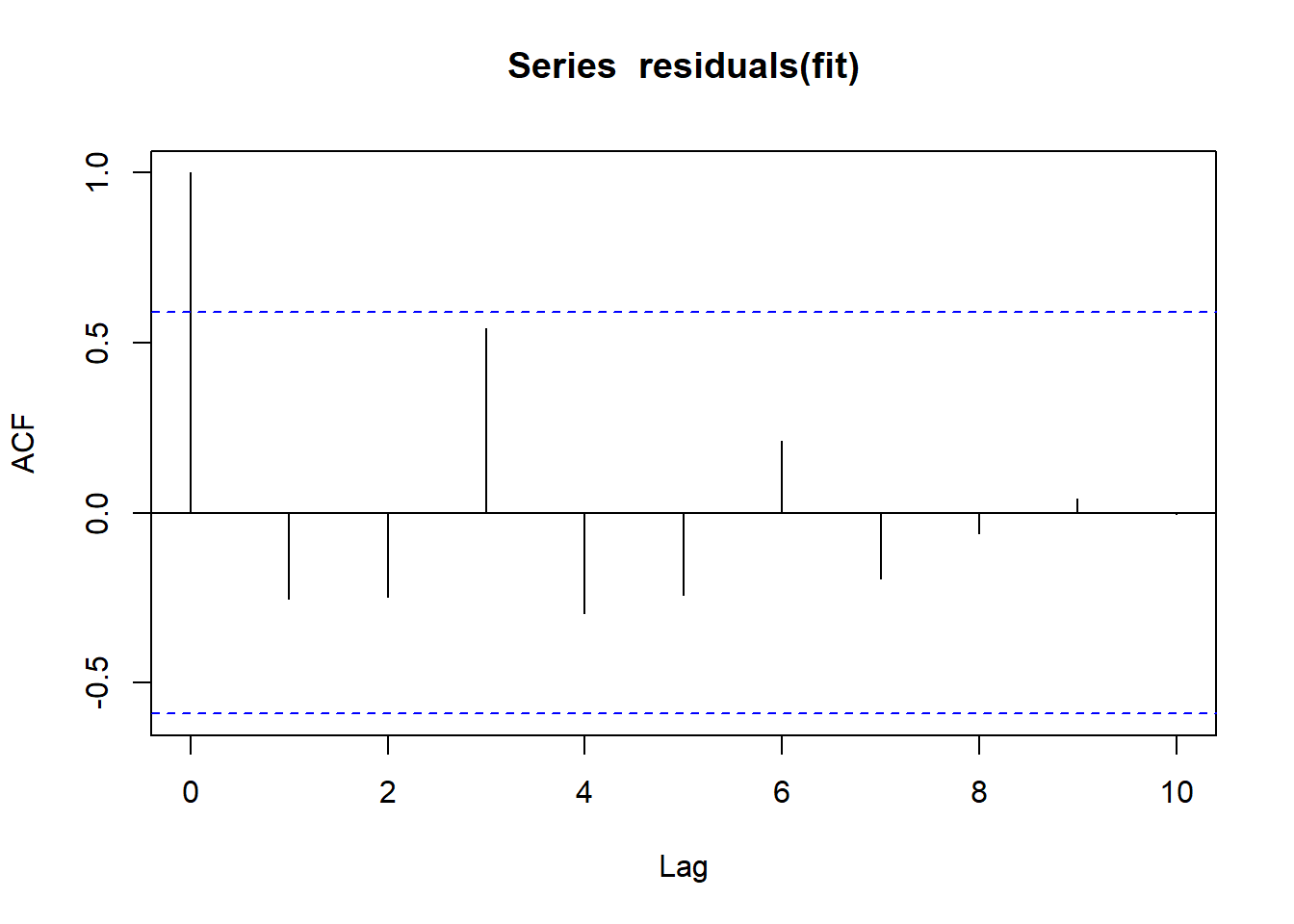

# nice wrapper function to generally test a lot of stuff
gvmodel <- gvlma(fit)
summary(gvmodel)


Call:
lm(formula = Weight_pre ~ Intervention + c.age + hispanic + c.stress, 
    data = mydata)

Residuals:
    Min      1Q  Median      3Q     Max 
-12.489  -6.318  -3.487   3.938  21.848 

Coefficients:
              Estimate Std. Error t value Pr(>|t|)    
(Intercept)   72.36794    7.12041  10.163 5.28e-05 ***
InterventionB  8.49465   13.23090   0.642    0.545    
c.age         -0.73751    3.05179  -0.242    0.817    
hispanic      -7.90293   10.31259  -0.766    0.473    
c.stress      -0.08953    1.37517  -0.065    0.950    
---
Signif. codes:  0 '***' 0.001 '**' 0.01 '*' 0.05 '.' 0.1 ' ' 1

Residual standard error: 12.77 on 6 degrees of freedom
Multiple R-squared:  0.1503,    Adjusted R-squared:  -0.4162 
F-statistic: 0.2652 on 4 and 6 DF,  p-value: 0.8902


ASSESSMENT OF THE LINEAR MODEL ASSUMPTIONS
USING THE GLOBAL TEST ON 4 DEGREES-OF-FREEDOM:
Level of Significance =  0.05 

Call:
 gvlma(x = fit) 

                     Value p-value                   Decision
Global Stat        8.79896 0.06633    Assumptions acceptable.
Skewness           1.68148 0.19473    Assumptions acceptable.
Kurtosis           0.01765 0.89431    Assumptions acceptable.
Link Function      4.82450 0.02806 Assumptions NOT satisfied!
Heteroscedasticity 2.27533 0.13145    Assumptions acceptable.

No significant differences.

Post Weight

Test for significant differences after intervention

# Post INtervention Weight - should beno difference
# not controls
fit <- lm(Weight_post ~ Intervention, mydata)
anova(fit)

Analysis of Variance Table

Response: Weight_post
             Df  Sum Sq Mean Sq F value Pr(>F)
Intervention  1   90.48  90.484  0.6896 0.4278
Residuals     9 1180.91 131.212

summary(fit)


Call:
lm(formula = Weight_post ~ Intervention, data = mydata)

Residuals:
   Min     1Q Median     3Q    Max 
-16.70  -7.43  -6.00   7.62  16.30 

Coefficients:
              Estimate Std. Error t value Pr(>|t|)    
(Intercept)     68.600      4.676   14.67 1.37e-07 ***
InterventionB    5.760      6.936    0.83    0.428    
---
Signif. codes:  0 '***' 0.001 '**' 0.01 '*' 0.05 '.' 0.1 ' ' 1

Residual standard error: 11.45 on 9 degrees of freedom
Multiple R-squared:  0.07117,   Adjusted R-squared:  -0.03203 
F-statistic: 0.6896 on 1 and 9 DF,  p-value: 0.4278

fit <- lm(Weight_post ~ Intervention + c.age + hispanic + c.stress,
          mydata)
anova(fit)

Analysis of Variance Table

Response: Weight_post
             Df  Sum Sq Mean Sq F value Pr(>F)
Intervention  1   90.48  90.484  0.5206 0.4977
c.age         1    4.00   4.003  0.0230 0.8843
hispanic      1  134.10 134.096  0.7716 0.4135
c.stress      1    0.07   0.066  0.0004 0.9851
Residuals     6 1042.75 173.791

summary(fit)


Call:
lm(formula = Weight_post ~ Intervention + c.age + hispanic + 
    c.stress, data = mydata)

Residuals:
    Min      1Q  Median      3Q     Max 
-12.702  -6.973  -3.441   3.527  21.626 

Coefficients:
              Estimate Std. Error t value Pr(>|t|)    
(Intercept)   72.35473    7.35115   9.843 6.34e-05 ***
InterventionB  9.64939   13.65965   0.706    0.506    
c.age         -1.32811    3.15069  -0.422    0.688    
hispanic      -8.67842   10.64678  -0.815    0.446    
c.stress       0.02763    1.41973   0.019    0.985    
---
Signif. codes:  0 '***' 0.001 '**' 0.01 '*' 0.05 '.' 0.1 ' ' 1

Residual standard error: 13.18 on 6 degrees of freedom
Multiple R-squared:  0.1798,    Adjusted R-squared:  -0.3669 
F-statistic: 0.3289 on 4 and 6 DF,  p-value: 0.8493

# diagnostic plots
layout(matrix(c(1,2,3,4),2,2)) # optional layout
plot(fit) # diagnostic plots

# normality again
shapiro.test(residuals(fit))


    Shapiro-Wilk normality test

data:  residuals(fit)
W = 0.91814, p-value = 0.3034

# independence
durbinWatsonTest(fit)

 lag Autocorrelation D-W Statistic p-value
   1      -0.3361658      2.610712   0.278
 Alternative hypothesis: rho != 0

layout(matrix(c(1),1,1))
acf(residuals(fit))

# nice wrapper function to generally test a lot of stuff
gvmodel <- gvlma(fit)
summary(gvmodel)


Call:
lm(formula = Weight_post ~ Intervention + c.age + hispanic + 
    c.stress, data = mydata)

Residuals:
    Min      1Q  Median      3Q     Max 
-12.702  -6.973  -3.441   3.527  21.626 

Coefficients:
              Estimate Std. Error t value Pr(>|t|)    
(Intercept)   72.35473    7.35115   9.843 6.34e-05 ***
InterventionB  9.64939   13.65965   0.706    0.506    
c.age         -1.32811    3.15069  -0.422    0.688    
hispanic      -8.67842   10.64678  -0.815    0.446    
c.stress       0.02763    1.41973   0.019    0.985    
---
Signif. codes:  0 '***' 0.001 '**' 0.01 '*' 0.05 '.' 0.1 ' ' 1

Residual standard error: 13.18 on 6 degrees of freedom
Multiple R-squared:  0.1798,    Adjusted R-squared:  -0.3669 
F-statistic: 0.3289 on 4 and 6 DF,  p-value: 0.8493


ASSESSMENT OF THE LINEAR MODEL ASSUMPTIONS
USING THE GLOBAL TEST ON 4 DEGREES-OF-FREEDOM:
Level of Significance =  0.05 

Call:
 gvlma(x = fit) 

                       Value  p-value                   Decision
Global Stat        11.687482 0.019833 Assumptions NOT satisfied!
Skewness            1.471559 0.225100    Assumptions acceptable.
Kurtosis            0.004073 0.949115    Assumptions acceptable.
Link Function       7.940367 0.004834 Assumptions NOT satisfied!
Heteroscedasticity  2.271483 0.131774    Assumptions acceptable.

Difference Scores of Weight

Test for significant differences after intervention

# Post INtervention Weight - should beno difference
# not controls
fit <- lm(Weight_diff ~ Intervention, mydata)
anova(fit)

Analysis of Variance Table

Response: Weight_diff
             Df Sum Sq Mean Sq F value Pr(>F)
Intervention  1  1.955  1.9550  0.5596 0.4735
Residuals     9 31.441  3.4935

summary(fit)


Call:
lm(formula = Weight_diff ~ Intervention, data = mydata)

Residuals:
    Min      1Q  Median      3Q     Max 
-3.8200 -0.9933  0.4800  1.2833  2.0800 

Coefficients:
              Estimate Std. Error t value Pr(>|t|)
(Intercept)     0.3667     0.7631   0.481    0.642
InterventionB  -0.8467     1.1318  -0.748    0.474

Residual standard error: 1.869 on 9 degrees of freedom
Multiple R-squared:  0.05854,   Adjusted R-squared:  -0.04607 
F-statistic: 0.5596 on 1 and 9 DF,  p-value: 0.4735

fit <- lm(Weight_diff ~ Intervention + c.age + hispanic + c.stress,
          mydata)
anova(fit)

Analysis of Variance Table

Response: Weight_diff
             Df  Sum Sq Mean Sq F value  Pr(>F)  
Intervention  1  1.9550  1.9550  0.8962 0.38036  
c.age         1 15.1063 15.1063  6.9245 0.03898 *
hispanic      1  2.0622  2.0622  0.9453 0.36847  
c.stress      1  1.1834  1.1834  0.5425 0.48919  
Residuals     6 13.0894  2.1816                  
---
Signif. codes:  0 '***' 0.001 '**' 0.01 '*' 0.05 '.' 0.1 ' ' 1

summary(fit)


Call:
lm(formula = Weight_diff ~ Intervention + c.age + hispanic + 
    c.stress, data = mydata)

Residuals:
    Min      1Q  Median      3Q     Max 
-1.9016 -0.7507 -0.0148  0.7534  1.6955 

Coefficients:
              Estimate Std. Error t value Pr(>|t|)
(Intercept)    0.01321    0.82362   0.016    0.988
InterventionB -1.15474    1.53042  -0.755    0.479
c.age          0.59060    0.35300   1.673    0.145
hispanic       0.77548    1.19286   0.650    0.540
c.stress      -0.11716    0.15907  -0.737    0.489

Residual standard error: 1.477 on 6 degrees of freedom
Multiple R-squared:  0.6081,    Adjusted R-squared:  0.3468 
F-statistic: 2.327 on 4 and 6 DF,  p-value: 0.17

results.diff[["Weight"]] <- summary(fit)[["coefficients"]]

# diagnostic plots
layout(matrix(c(1,2,3,4),2,2)) # optional layout
plot(fit) # diagnostic plots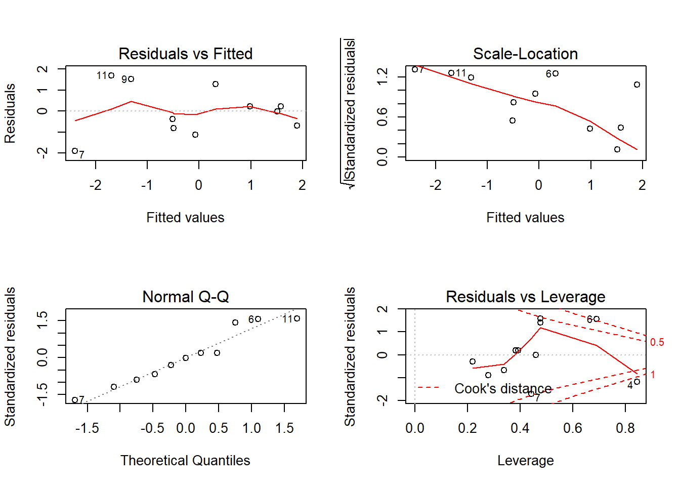

# normality again
shapiro.test(residuals(fit))


    Shapiro-Wilk normality test

data:  residuals(fit)
W = 0.95573, p-value = 0.7175

# independence
durbinWatsonTest(fit)

 lag Autocorrelation D-W Statistic p-value
   1      0.00132079      1.727779   0.722
 Alternative hypothesis: rho != 0

layout(matrix(c(1),1,1))
acf(residuals(fit))

# nice wrapper function to generally test a lot of stuff
gvmodel <- gvlma(fit)
summary(gvmodel)


Call:
lm(formula = Weight_diff ~ Intervention + c.age + hispanic + 
    c.stress, data = mydata)

Residuals:
    Min      1Q  Median      3Q     Max 
-1.9016 -0.7507 -0.0148  0.7534  1.6955 

Coefficients:
              Estimate Std. Error t value Pr(>|t|)
(Intercept)    0.01321    0.82362   0.016    0.988
InterventionB -1.15474    1.53042  -0.755    0.479
c.age          0.59060    0.35300   1.673    0.145
hispanic       0.77548    1.19286   0.650    0.540
c.stress      -0.11716    0.15907  -0.737    0.489

Residual standard error: 1.477 on 6 degrees of freedom
Multiple R-squared:  0.6081,    Adjusted R-squared:  0.3468 
F-statistic: 2.327 on 4 and 6 DF,  p-value: 0.17


ASSESSMENT OF THE LINEAR MODEL ASSUMPTIONS
USING THE GLOBAL TEST ON 4 DEGREES-OF-FREEDOM:
Level of Significance =  0.05 

Call:
 gvlma(x = fit) 

                     Value p-value                Decision
Global Stat        2.13957  0.7101 Assumptions acceptable.
Skewness           0.01451  0.9041 Assumptions acceptable.
Kurtosis           0.42946  0.5123 Assumptions acceptable.
Link Function      0.94668  0.3306 Assumptions acceptable.
Heteroscedasticity 0.74893  0.3868 Assumptions acceptable.

Therefore, we have evidence that weight (kg) is not effected by Prebiotic vs. placebo.

Results Adjusted for Multiple Comparisons

all_results <- unlist.res(results.diff)

Joining, by = c("Estimate", "Std. Error", "t value", "Pr(>|t|)", "Outcome", "Parameter")
Joining, by = c("Estimate", "Std. Error", "t value", "Pr(>|t|)", "Outcome", "Parameter")
Joining, by = c("Estimate", "Std. Error", "t value", "Pr(>|t|)", "Outcome", "Parameter")

all_results$p.adj <- p.adjust(all_results$`Pr(>|t|)`, "fdr") 
all_results$sigflag <- ifelse(all_results$p.adj < 0.05, "*", " ")
all_results$`Pr(>|t|)` <- round(all_results$`Pr(>|t|)`, 3)
all_results$p.adj.fdr <- round(all_results$p.adj, 3)
all_results <- all_results[,c(5:6, 1:4,7:8)]

kable(all_results, format="html", digits=3) %>%
  kable_styling(full_width = T)

Outcome	Parameter	Estimate	Std. Error	t value	Pr(>\|t\|)	p.adj
BMI	(Intercept)	0.004	0.295	0.014	0.989	0.989
BMI	InterventionB	-0.419	0.549	-0.764	0.474	0.789
BMI	c.age	0.219	0.127	1.730	0.134	0.581
BMI	hispanic	0.283	0.428	0.661	0.533	0.789
BMI	c.stress	-0.034	0.057	-0.604	0.568	0.789
LBM	(Intercept)	-0.223	0.452	-0.492	0.640	0.789
LBM	InterventionB	0.620	0.840	0.738	0.489	0.789
LBM	c.age	0.093	0.194	0.478	0.650	0.789
LBM	hispanic	-0.293	0.655	-0.447	0.670	0.789
LBM	c.stress	-0.053	0.087	-0.606	0.567	0.789
VFL	(Intercept)	-0.174	0.366	-0.475	0.652	0.789
VFL	InterventionB	-1.576	0.681	-2.314	0.060	0.480
VFL	c.age	0.342	0.157	2.180	0.072	0.480
VFL	hispanic	1.685	0.531	3.174	0.019	0.384
VFL	c.stress	0.001	0.071	0.015	0.989	0.989
Weight	(Intercept)	0.013	0.824	0.016	0.988	0.989
Weight	InterventionB	-1.155	1.530	-0.755	0.479	0.789
Weight	c.age	0.591	0.353	1.673	0.145	0.581
Weight	hispanic	0.775	1.193	0.650	0.540	0.789
Weight	c.stress	-0.117	0.159	-0.737	0.489	0.789

readr::write_csv(all_results, "tab/results_anthropometric.csv")

sessionInfo()

R version 3.6.3 (2020-02-29)
Platform: x86_64-w64-mingw32/x64 (64-bit)
Running under: Windows 10 x64 (build 18362)

Matrix products: default

locale:
[1] LC_COLLATE=English_United States.1252 
[2] LC_CTYPE=English_United States.1252   
[3] LC_MONETARY=English_United States.1252
[4] LC_NUMERIC=C                          
[5] LC_TIME=English_United States.1252    

attached base packages:
[1] stats     graphics  grDevices utils     datasets  methods   base     

other attached packages:
 [1] cowplot_1.0.0     microbiome_1.8.0  car_3.0-8         carData_3.0-4    
 [5] gvlma_1.0.0.3     patchwork_1.0.0   viridis_0.5.1     viridisLite_0.3.0
 [9] gridExtra_2.3     xtable_1.8-4      kableExtra_1.1.0  plyr_1.8.6       
[13] data.table_1.12.8 readxl_1.3.1      forcats_0.5.0     stringr_1.4.0    
[17] dplyr_0.8.5       purrr_0.3.4       readr_1.3.1       tidyr_1.1.0      
[21] tibble_3.0.1      ggplot2_3.3.0     tidyverse_1.3.0   lmerTest_3.1-2   
[25] lme4_1.1-23       Matrix_1.2-18     vegan_2.5-6       lattice_0.20-38  
[29] permute_0.9-5     phyloseq_1.30.0  

loaded via a namespace (and not attached):
 [1] Rtsne_0.15          minqa_1.2.4         colorspace_1.4-1   
 [4] rio_0.5.16          ellipsis_0.3.1      rprojroot_1.3-2    
 [7] XVector_0.26.0      fs_1.4.1            rstudioapi_0.11    
[10] farver_2.0.3        fansi_0.4.1         lubridate_1.7.8    
[13] xml2_1.3.2          codetools_0.2-16    splines_3.6.3      
[16] knitr_1.28          ade4_1.7-15         jsonlite_1.6.1     
[19] workflowr_1.6.2     nloptr_1.2.2.1      broom_0.5.6        
[22] cluster_2.1.0       dbplyr_1.4.4        BiocManager_1.30.10
[25] compiler_3.6.3      httr_1.4.1          backports_1.1.7    
[28] assertthat_0.2.1    cli_2.0.2           later_1.0.0        
[31] htmltools_0.4.0     tools_3.6.3         igraph_1.2.5       
[34] gtable_0.3.0        glue_1.4.1          reshape2_1.4.4     
[37] Rcpp_1.0.4.6        Biobase_2.46.0      cellranger_1.1.0   
[40] vctrs_0.3.0         Biostrings_2.54.0   multtest_2.42.0    
[43] ape_5.3             nlme_3.1-144        iterators_1.0.12   
[46] xfun_0.14           openxlsx_4.1.5      rvest_0.3.5        
[49] lifecycle_0.2.0     statmod_1.4.34      zlibbioc_1.32.0    
[52] MASS_7.3-51.5       scales_1.1.1        hms_0.5.3          
[55] promises_1.1.0      parallel_3.6.3      biomformat_1.14.0  
[58] rhdf5_2.30.1        curl_4.3            yaml_2.2.1         
[61] stringi_1.4.6       highr_0.8           S4Vectors_0.24.4   
[64] foreach_1.5.0       BiocGenerics_0.32.0 zip_2.0.4          
[67] boot_1.3-24         rlang_0.4.6         pkgconfig_2.0.3    
[70] evaluate_0.14       Rhdf5lib_1.8.0      labeling_0.3       
[73] tidyselect_1.1.0    magrittr_1.5        R6_2.4.1           
[76] IRanges_2.20.2      generics_0.0.2      DBI_1.1.0          
[79] foreign_0.8-75      pillar_1.4.4        haven_2.3.0        
[82] whisker_0.4         withr_2.2.0         mgcv_1.8-31        
[85] abind_1.4-5         survival_3.1-8      modelr_0.1.8       
[88] crayon_1.3.4        rmarkdown_2.1       grid_3.6.3         
[91] blob_1.2.1          git2r_0.27.1        reprex_0.3.0       
[94] digest_0.6.25       webshot_0.5.2       httpuv_1.5.2       
[97] numDeriv_2016.8-1.1 stats4_3.6.3        munsell_0.5.0

Anthropometric Analyses

Overview of aims

Analyses

BMI

Pre BMI

Post BMI

Difference Scores of BMI

Figure 6 changes in BMI

Lean Body Mass (LBM)

Pre LBM

Post LBM

Difference Scores of LBM

Visceral Fat Level (VFL) Fat Mass

Pre VFL

Post VFL

Difference Scores of VFL

Weight (kg)

Pre Weight

Post Weight

Difference Scores of Weight

Results Adjusted for Multiple Comparisons