Blood Data Analyses
Last updated: 2020-06-08
Checks: 7 0
Knit directory: Fiber_Intervention_Study/
This reproducible R Markdown analysis was created with workflowr (version 1.6.2). The Checks tab describes the reproducibility checks that were applied when the results were created. The Past versions tab lists the development history.
Great! Since the R Markdown file has been committed to the Git repository, you know the exact version of the code that produced these results.
Great job! The global environment was empty. Objects defined in the global environment can affect the analysis in your R Markdown file in unknown ways. For reproduciblity it’s best to always run the code in an empty environment.
The command set.seed(20191210) was run prior to running the code in the R Markdown file. Setting a seed ensures that any results that rely on randomness, e.g. subsampling or permutations, are reproducible.
Great job! Recording the operating system, R version, and package versions is critical for reproducibility.
Nice! There were no cached chunks for this analysis, so you can be confident that you successfully produced the results during this run.
Great job! Using relative paths to the files within your workflowr project makes it easier to run your code on other machines.
Great! You are using Git for version control. Tracking code development and connecting the code version to the results is critical for reproducibility.
The results in this page were generated with repository version 94015da. See the Past versions tab to see a history of the changes made to the R Markdown and HTML files.
Note that you need to be careful to ensure that all relevant files for the analysis have been committed to Git prior to generating the results (you can use wflow_publish or wflow_git_commit). workflowr only checks the R Markdown file, but you know if there are other scripts or data files that it depends on. Below is the status of the Git repository when the results were generated:
Ignored files:
    Ignored:    .Rhistory
    Ignored:    .Rproj.user/
    Ignored:    code/.Rhistory
    Ignored:    reference-papers/Dietary_Variables.xlsx
    Ignored:    reference-papers/Johnson_2019.pdf

Untracked files:
    Untracked:  fig/fig/
    Untracked:  fig/figure-2020-06-01/
    Untracked:  fig/figure2.pdf
    Untracked:  fig/figure3.pdf
    Untracked:  fig/figure5_glmm.pdf
    Untracked:  fig/figure6.pdf
    Untracked:  fig/figures-2020-06-08.zip
    Untracked:  fig/figures-2020-06-08/
    Untracked:  renv/
    Untracked:  tab/figure6_data_change_BMI.csv
    Untracked:  tab/sample_size_summary.xlsx
    Untracked:  tab/table_1_results.csv
Note that any generated files, e.g. HTML, png, CSS, etc., are not included in this status report because it is ok for generated content to have uncommitted changes.
These are the previous versions of the repository in which changes were made to the R Markdown (analysis/analysis_blood_data.Rmd) and HTML (docs/analysis_blood_data.html) files. If you’ve configured a remote Git repository (see ?wflow_git_remote), click on the hyperlinks in the table below to view the files as they were in that past version.
| File | Version | Author | Date | Message |
|---|---|---|---|---|
| Rmd | 94015da | noah-padgett | 2020-06-08 | revised figures |
| html | 94015da | noah-padgett | 2020-06-08 | revised figures |
| html | 0733fe5 | noah-padgett | 2020-05-21 | Build site. |
| Rmd | d576bdd | noah-padgett | 2020-05-21 | tables outputted |
| html | d576bdd | noah-padgett | 2020-05-21 | tables outputted |
| Rmd | ef7cab9 | noah-padgett | 2020-05-14 | blood measure analyses |
| html | ef7cab9 | noah-padgett | 2020-05-14 | blood measure analyses |
Overview of aims
What is the effect of Prebiotin vs placebo on blood measures (controlling for diet, age, ethnicity, stress?) Did the intervention effect?
Data
blood_data <- read_excel("data/Blood measures data/Copy of Fiber Study Blood Results.xlsx")

meta_data <- microbiome_data$meta.dat

keepVar <- c("SubjectID", "Week", "Intervention", "Stress.Scale", "Ethnicity", "Gender", "Age")
meta_data <- meta_data [, keepVar] %>%
  filter(Week == 1)

mydata <- full_join(blood_data, meta_data)
Joining, by = "SubjectID"# recoding
mydata <- mydata %>%
mutate(female = ifelse(Gender == "F", 1, 0),
c.age = Age - mean(Age),
IntB = ifelse(Intervention == "B", 1, 0),
Post = ifelse(time == "Post", 1, 0),
c.stress = Stress.Scale - mean(Stress.Scale),
hispanic = ifelse(Ethnicity %in% c("White", "Asian", "Native America"), 1, 0))
# for plotting
plot.data <- mydata[, c(colnames(mydata)[c(1:18,20:24)])]
plot.data <- plot.data %>%
pivot_longer(cols=colnames(mydata)[3:18],
names_to = "Variable",
values_to = "value")Data summary
Summary Statistics
varNames <- c(colnames(mydata)[c(2:18,20)])

sum.dat <- mydata[,varNames[2:17]] %>%
  summarise_all(list(Mean=mean, SD=sd,
                     min=min, Median=median, Max=max))
sum.dat <- data.frame(matrix(unlist(sum.dat), ncol=5))
colnames(sum.dat) <- c("Mean", "SD", "Min", "Median", "Max")
rownames(sum.dat) <- varNames[2:17]

kable(sum.dat, format="html", digits=3)%>%
kable_styling(full_width = T)| Mean | SD | Min | Median | Max | |
|---|---|---|---|---|---|
| Glucose | 93.591 | 8.857 | 84.00 | 93.500 | 128.00 |
| BUN | 12.636 | 2.194 | 7.00 | 12.500 | 16.00 |
| Creatinine | 0.820 | 0.088 | 0.61 | 0.820 | 0.99 |
| Sodium | 141.682 | 1.810 | 138.00 | 142.000 | 145.00 |
| Potassium | 4.400 | 0.393 | 3.70 | 4.300 | 5.70 |
| Chloride | 102.500 | 1.871 | 99.00 | 102.500 | 107.00 |
| Carbon_Dioxide | 24.955 | 2.299 | 21.00 | 25.500 | 30.00 |
| Calcium | 9.327 | 0.319 | 8.70 | 9.300 | 9.80 |
| Cholesterol | 180.409 | 39.740 | 118.00 | 179.500 | 261.00 |
| Triglycerides | 116.864 | 90.611 | 46.00 | 96.500 | 415.00 |
| HDL | 60.091 | 14.671 | 37.00 | 59.000 | 96.00 |
| LDL | 97.577 | 33.402 | 45.00 | 87.000 | 171.00 |
| LDL_HDL_Ratio | 1.697 | 0.771 | 0.63 | 1.365 | 3.45 |
| hsCRP | 1.973 | 2.466 | 0.30 | 0.900 | 10.70 |
| Insulin | 17.091 | 27.233 | 3.00 | 8.000 | 101.00 |
| PYY | 103.329 | 175.191 | 16.56 | 36.215 | 742.90 |
Summary of these data by Intervention Group
varNames <- colnames(mydata)[c(20,3:18)]
sum.dat <- mydata[,varNames] %>%
  group_by(Intervention) %>%
  summarise_all(list(Mean=mean, SD=sd,
                     min=min, Median=median, Max=max))

a <- data.frame(matrix(unlist(sum.dat[1,-1]), ncol=5))
b <- data.frame(matrix(unlist(sum.dat[2,-1]), ncol=5))
a <- cbind(rep("A", 16), a); colnames(a) <- c("Intervention", "Mean", "SD", "Min", "Median", "Max")
b <- cbind(rep("B", 16), b); colnames(b) <- c("Intervention", "Mean", "SD", "Min", "Median", "Max")

sum.dat <- rbind(a,b)
sum.dat <- data.frame(Variable=rep(varNames[-1],2), sum.dat)

sum.dat <- arrange(sum.dat, Variable)
kable(sum.dat, format="html", digits=3)%>%
kable_styling(full_width = T)| Variable | Intervention | Mean | SD | Min | Median | Max |
|---|---|---|---|---|---|---|
| BUN | A | 12.333 | 2.674 | 7.00 | 12.500 | 16.00 |
| BUN | B | 13.000 | 1.491 | 11.00 | 12.500 | 16.00 |
| Calcium | A | 9.258 | 0.401 | 8.70 | 9.300 | 9.80 |
| Calcium | B | 9.410 | 0.166 | 9.20 | 9.350 | 9.70 |
| Carbon_Dioxide | A | 24.833 | 2.691 | 21.00 | 25.500 | 30.00 |
| Carbon_Dioxide | B | 25.100 | 1.853 | 22.00 | 25.500 | 28.00 |
| Chloride | A | 102.500 | 1.931 | 101.00 | 102.000 | 107.00 |
| Chloride | B | 102.500 | 1.900 | 99.00 | 102.500 | 105.00 |
| Cholesterol | A | 160.667 | 25.921 | 118.00 | 160.500 | 198.00 |
| Cholesterol | B | 204.100 | 41.479 | 137.00 | 203.000 | 261.00 |
| Creatinine | A | 0.798 | 0.086 | 0.61 | 0.810 | 0.92 |
| Creatinine | B | 0.847 | 0.087 | 0.72 | 0.845 | 0.99 |
| Glucose | A | 91.500 | 4.317 | 84.00 | 92.000 | 97.00 |
| Glucose | B | 96.100 | 12.142 | 84.00 | 93.500 | 128.00 |
| HDL | A | 63.083 | 13.780 | 43.00 | 59.000 | 96.00 |
| HDL | B | 56.500 | 15.615 | 37.00 | 55.500 | 80.00 |
| hsCRP | A | 2.058 | 2.863 | 0.30 | 0.900 | 10.70 |
| hsCRP | B | 1.870 | 2.037 | 0.40 | 1.150 | 7.00 |
| Insulin | A | 8.333 | 5.836 | 3.00 | 7.500 | 26.00 |
| Insulin | B | 27.600 | 38.260 | 7.00 | 9.000 | 101.00 |
| LDL | A | 82.500 | 23.209 | 45.00 | 80.500 | 117.00 |
| LDL | B | 115.670 | 35.750 | 65.00 | 114.500 | 171.00 |
| LDL_HDL_Ratio | A | 1.383 | 0.583 | 0.63 | 1.255 | 2.72 |
| LDL_HDL_Ratio | B | 2.075 | 0.825 | 1.27 | 1.835 | 3.45 |
| Potassium | A | 4.442 | 0.425 | 4.10 | 4.300 | 5.70 |
| Potassium | B | 4.350 | 0.366 | 3.70 | 4.350 | 4.90 |
| PYY | A | 141.648 | 229.661 | 22.62 | 39.075 | 742.90 |
| PYY | B | 57.345 | 53.314 | 16.56 | 36.215 | 161.80 |
| Sodium | A | 140.917 | 1.443 | 138.00 | 141.000 | 143.00 |
| Sodium | B | 142.600 | 1.838 | 138.00 | 143.000 | 145.00 |
| Triglycerides | A | 75.250 | 31.792 | 46.00 | 60.000 | 132.00 |
| Triglycerides | B | 166.800 | 113.325 | 57.00 | 120.000 | 415.00 |
Summary of these data by Pre-Post
varNames <- colnames(mydata)[c(2:18)]

sum.dat <- mydata[,varNames] %>%
  group_by(time) %>%
  summarise_all(list(Mean=mean, SD=sd,
                     min=min, Median=median, Max=max))

a <- data.frame(matrix(unlist(sum.dat[1,-1]), ncol=5))
b <- data.frame(matrix(unlist(sum.dat[2,-1]), ncol=5))
a <- cbind(rep("Post", 16), a); colnames(a) <- c("Pre-Post", "Mean", "SD", "Min", "Median", "Max")
b <- cbind(rep("Pre", 16), b); colnames(b) <- c("Pre-Post", "Mean", "SD", "Min", "Median", "Max")

sum.dat <- rbind(b,a)
sum.dat <- data.frame(Variable=rep(varNames[-1],2), sum.dat)

sum.dat <- arrange(sum.dat, Variable)
kable(sum.dat, format="html", digits=3)%>%
kable_styling(full_width = T)| Variable | Pre.Post | Mean | SD | Min | Median | Max |
|---|---|---|---|---|---|---|
| BUN | Pre | 12.455 | 2.734 | 7.00 | 13.00 | 16.00 |
| BUN | Post | 12.818 | 1.601 | 11.00 | 12.00 | 16.00 |
| Calcium | Pre | 9.155 | 0.327 | 8.70 | 9.20 | 9.80 |
| Calcium | Post | 9.500 | 0.205 | 9.30 | 9.40 | 9.80 |
| Carbon_Dioxide | Pre | 24.182 | 2.040 | 21.00 | 24.00 | 27.00 |
| Carbon_Dioxide | Post | 25.727 | 2.370 | 21.00 | 26.00 | 30.00 |
| Chloride | Pre | 103.000 | 1.789 | 101.00 | 103.00 | 107.00 |
| Chloride | Post | 102.000 | 1.897 | 99.00 | 101.00 | 105.00 |
| Cholesterol | Pre | 175.636 | 42.601 | 130.00 | 162.00 | 253.00 |
| Cholesterol | Post | 185.182 | 38.099 | 118.00 | 190.00 | 261.00 |
| Creatinine | Pre | 0.798 | 0.097 | 0.61 | 0.78 | 0.94 |
| Creatinine | Post | 0.842 | 0.076 | 0.72 | 0.82 | 0.99 |
| Glucose | Pre | 92.364 | 4.905 | 84.00 | 94.00 | 100.00 |
| Glucose | Post | 94.818 | 11.720 | 84.00 | 93.00 | 128.00 |
| HDL | Pre | 56.455 | 12.668 | 40.00 | 58.00 | 75.00 |
| HDL | Post | 63.727 | 16.199 | 37.00 | 64.00 | 96.00 |
| hsCRP | Pre | 2.255 | 2.935 | 0.40 | 1.50 | 10.70 |
| hsCRP | Post | 1.691 | 1.995 | 0.30 | 0.80 | 7.00 |
| Insulin | Pre | 15.818 | 27.633 | 4.00 | 8.00 | 99.00 |
| Insulin | Post | 18.364 | 28.111 | 3.00 | 8.00 | 101.00 |
| LDL | Pre | 96.545 | 38.435 | 45.00 | 85.00 | 171.00 |
| LDL | Post | 98.609 | 29.382 | 52.00 | 97.70 | 158.00 |
| LDL_HDL_Ratio | Pre | 1.838 | 0.946 | 0.63 | 1.39 | 3.45 |
| LDL_HDL_Ratio | Post | 1.556 | 0.555 | 0.81 | 1.34 | 2.67 |
| Potassium | Pre | 4.482 | 0.513 | 3.70 | 4.40 | 5.70 |
| Potassium | Post | 4.318 | 0.214 | 3.90 | 4.30 | 4.70 |
| PYY | Pre | 113.258 | 212.705 | 17.93 | 34.24 | 742.90 |
| PYY | Post | 93.399 | 137.814 | 16.56 | 38.19 | 490.10 |
| Sodium | Pre | 142.091 | 1.446 | 140.00 | 142.00 | 145.00 |
| Sodium | Post | 141.273 | 2.102 | 138.00 | 142.00 | 144.00 |
| Triglycerides | Pre | 113.636 | 78.834 | 48.00 | 107.00 | 322.00 |
| Triglycerides | Post | 120.091 | 104.900 | 46.00 | 86.00 | 415.00 |
Summary of these data by Intervention & Pre-Post
varNames <- colnames(mydata)[c(20, 2:18)]

sum.dat <- mydata[,varNames] %>%
  group_by(Intervention, time) %>%
  summarise_all(list(Mean=mean, SD=sd,
                     min=min, Median=median, Max=max))

a2 <- data.frame(matrix(unlist(sum.dat[1,-c(1:2)]), ncol=5))
a1 <- data.frame(matrix(unlist(sum.dat[2,-c(1:2)]), ncol=5))
b1 <- data.frame(matrix(unlist(sum.dat[3,-c(1:2)]), ncol=5))
b2 <- data.frame(matrix(unlist(sum.dat[4,-c(1:2)]), ncol=5))

a2 <- cbind(rep("A", 16), rep("Post", 16), a2); colnames(a2) <- c("Intervention", "Pre-Post", "Mean", "SD", "Min", "Median", "Max")
a1 <- cbind(rep("A", 16), rep("Pre", 16), a1); colnames(a1) <- c("Intervention", "Pre-Post", "Mean", "SD", "Min", "Median", "Max")

b1 <- cbind(rep("B", 16), rep("Pre", 16), b1); colnames(b1) <- c("Intervention", "Pre-Post", "Mean", "SD", "Min", "Median", "Max")

b2 <- cbind(rep("B", 16), rep("Post", 16), b2); colnames(b2) <- c("Intervention", "Pre-Post", "Mean", "SD", "Min", "Median", "Max")

sum.dat <- rbind(a1,a2, b1, b2)
sum.dat <- data.frame(Variable=rep(varNames[-c(1:2)],4), sum.dat)

sum.dat <- arrange(sum.dat, Variable)
kable(sum.dat, format="html", digits=3)%>%
kable_styling(full_width = T)| Variable | Intervention | Pre.Post | Mean | SD | Min | Median | Max |
|---|---|---|---|---|---|---|---|
| BUN | A | Pre | 11.333 | 3.141 | 7.00 | 11.500 | 16.00 |
| BUN | A | Post | 13.333 | 1.862 | 11.00 | 13.000 | 16.00 |
| BUN | B | Pre | 12.200 | 1.095 | 11.00 | 12.000 | 14.00 |
| BUN | B | Post | 13.800 | 1.483 | 12.00 | 14.000 | 16.00 |
| Calcium | A | Pre | 9.017 | 0.397 | 8.70 | 8.900 | 9.80 |
| Calcium | A | Post | 9.500 | 0.237 | 9.30 | 9.400 | 9.80 |
| Calcium | B | Pre | 9.500 | 0.187 | 9.30 | 9.600 | 9.70 |
| Calcium | B | Post | 9.320 | 0.084 | 9.20 | 9.300 | 9.40 |
| Carbon_Dioxide | A | Pre | 23.833 | 2.229 | 21.00 | 23.000 | 27.00 |
| Carbon_Dioxide | A | Post | 25.833 | 2.927 | 21.00 | 26.000 | 30.00 |
| Carbon_Dioxide | B | Pre | 25.600 | 1.817 | 23.00 | 26.000 | 28.00 |
| Carbon_Dioxide | B | Post | 24.600 | 1.949 | 22.00 | 24.000 | 27.00 |
| Chloride | A | Pre | 103.333 | 2.338 | 101.00 | 103.000 | 107.00 |
| Chloride | A | Post | 101.667 | 1.033 | 101.00 | 101.000 | 103.00 |
| Chloride | B | Pre | 102.400 | 2.702 | 99.00 | 104.000 | 105.00 |
| Chloride | B | Post | 102.600 | 0.894 | 102.00 | 102.000 | 104.00 |
| Cholesterol | A | Pre | 155.333 | 21.332 | 130.00 | 151.000 | 185.00 |
| Cholesterol | A | Post | 166.000 | 30.900 | 118.00 | 173.000 | 198.00 |
| Cholesterol | B | Pre | 208.200 | 34.946 | 165.00 | 205.000 | 261.00 |
| Cholesterol | B | Post | 200.000 | 51.069 | 137.00 | 201.000 | 253.00 |
| Creatinine | A | Pre | 0.760 | 0.100 | 0.61 | 0.770 | 0.89 |
| Creatinine | A | Post | 0.835 | 0.055 | 0.77 | 0.820 | 0.92 |
| Creatinine | B | Pre | 0.850 | 0.103 | 0.72 | 0.850 | 0.99 |
| Creatinine | B | Post | 0.844 | 0.081 | 0.76 | 0.840 | 0.94 |
| Glucose | A | Pre | 93.333 | 3.983 | 87.00 | 95.000 | 97.00 |
| Glucose | A | Post | 89.667 | 4.131 | 84.00 | 88.500 | 95.00 |
| Glucose | B | Pre | 101.000 | 15.313 | 91.00 | 95.000 | 128.00 |
| Glucose | B | Post | 91.200 | 6.099 | 84.00 | 90.000 | 100.00 |
| HDL | A | Pre | 60.000 | 11.730 | 43.00 | 59.000 | 75.00 |
| HDL | A | Post | 66.167 | 16.043 | 52.00 | 62.000 | 96.00 |
| HDL | B | Pre | 60.800 | 17.740 | 37.00 | 64.000 | 80.00 |
| HDL | B | Post | 52.200 | 13.700 | 40.00 | 47.000 | 71.00 |
| hsCRP | A | Pre | 3.000 | 3.873 | 0.50 | 1.850 | 10.70 |
| hsCRP | A | Post | 1.117 | 0.952 | 0.30 | 0.800 | 3.00 |
| hsCRP | B | Pre | 2.380 | 2.781 | 0.50 | 0.800 | 7.00 |
| hsCRP | B | Post | 1.360 | 0.976 | 0.40 | 1.500 | 2.80 |
| Insulin | A | Pre | 7.000 | 1.789 | 4.00 | 7.500 | 9.00 |
| Insulin | A | Post | 9.667 | 8.214 | 3.00 | 7.500 | 26.00 |
| Insulin | B | Pre | 28.800 | 40.518 | 7.00 | 12.000 | 101.00 |
| Insulin | B | Post | 26.400 | 40.599 | 7.00 | 8.000 | 99.00 |
| LDL | A | Pre | 79.167 | 24.203 | 45.00 | 78.500 | 117.00 |
| LDL | A | Post | 85.833 | 23.928 | 52.00 | 80.500 | 114.00 |
| LDL | B | Pre | 113.940 | 30.065 | 84.00 | 99.000 | 158.00 |
| LDL | B | Post | 117.400 | 44.320 | 65.00 | 130.000 | 171.00 |
| LDL_HDL_Ratio | A | Pre | 1.410 | 0.697 | 0.63 | 1.255 | 2.72 |
| LDL_HDL_Ratio | A | Post | 1.355 | 0.510 | 0.81 | 1.290 | 2.20 |
| LDL_HDL_Ratio | B | Pre | 1.798 | 0.558 | 1.31 | 1.700 | 2.67 |
| LDL_HDL_Ratio | B | Post | 2.352 | 1.014 | 1.27 | 2.400 | 3.45 |
| Potassium | A | Pre | 4.550 | 0.589 | 4.10 | 4.350 | 5.70 |
| Potassium | A | Post | 4.333 | 0.151 | 4.10 | 4.300 | 4.50 |
| Potassium | B | Pre | 4.300 | 0.292 | 3.90 | 4.300 | 4.70 |
| Potassium | B | Post | 4.400 | 0.458 | 3.70 | 4.400 | 4.90 |
| PYY | A | Pre | 157.692 | 287.213 | 23.44 | 38.995 | 742.90 |
| PYY | A | Post | 125.605 | 181.461 | 22.62 | 54.815 | 490.10 |
| PYY | B | Pre | 54.752 | 53.844 | 16.56 | 38.190 | 149.00 |
| PYY | B | Post | 59.938 | 58.985 | 17.93 | 34.240 | 161.80 |
| Sodium | A | Pre | 141.167 | 0.983 | 140.00 | 141.500 | 142.00 |
| Sodium | A | Post | 140.667 | 1.862 | 138.00 | 141.000 | 143.00 |
| Sodium | B | Pre | 142.000 | 2.345 | 138.00 | 143.000 | 144.00 |
| Sodium | B | Post | 143.200 | 1.095 | 142.00 | 143.000 | 145.00 |
| Triglycerides | A | Pre | 80.833 | 37.965 | 48.00 | 64.000 | 132.00 |
| Triglycerides | A | Post | 69.667 | 26.598 | 46.00 | 59.500 | 118.00 |
| Triglycerides | B | Pre | 180.600 | 135.038 | 86.00 | 116.000 | 415.00 |
| Triglycerides | B | Post | 153.000 | 100.918 | 57.00 | 124.000 | 322.00 |
Analysis
Next, the aim is to more formally test for differences between intervention groups.
# plot
p1 <- ggplot(plot.data,
             aes(x=time, y=value, group=time, color=time))+
  geom_boxplot(outlier.shape = NA)+
  geom_jitter(width = 0.25)+
  facet_wrap(.~Variable, scales = "free") +
  labs(x=NULL, title="Pre and Post Blood Measures")+
  theme(panel.grid = element_blank(),
        axis.text = element_text(size=10))
p1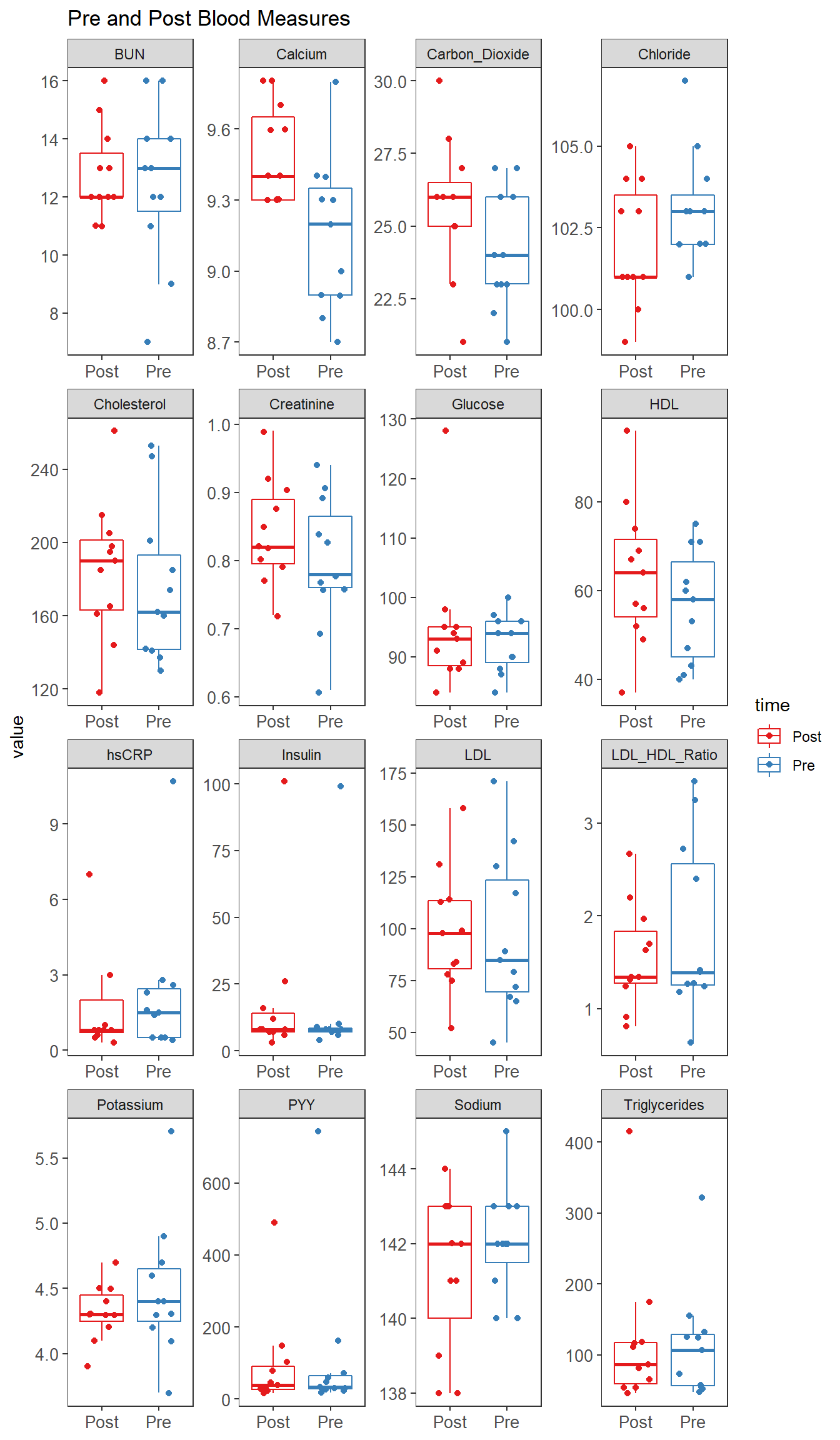
p2 <- ggplot(plot.data,
             aes(x=time, y=value, group=time, color=time))+
  geom_boxplot(outlier.shape = NA)+
  geom_jitter(width = 0.25, size=2)+
  labs(x=NULL,y=NULL, title="Blood Measures by Time & Intervention Group")+
  facet_grid(Variable~Intervention, scale="free", labeller = labeller(Intervention = c(A = "Group A", B = "Group B")))+
  theme(panel.grid = element_blank(),
        axis.text = element_text(size=10),
        strip.text = element_text(size=10))
p2
Run Analyses
This is simply to double check that no differences occured at baseline.
results.out <- list()
i <- 1
varNames <- colnames(mydata)[3:18]
for(i in 1:length(varNames)){
cat("\n\n=======================")
cat("\n=======================")
cat("\nOutcome:\t",varNames[i])
cat("\n")
form <- as.formula(paste0(varNames[i], "~ IntB + Post + IntB:Post + c.age"))
fit <- lm(form, mydata)
anova(fit)
results.out[[varNames[i]]] <- summary(fit)[["coefficients"]]
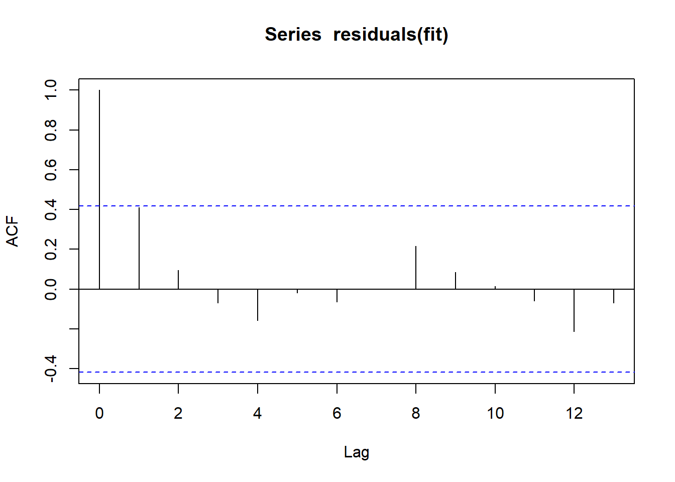
# diagnostic plots
layout(matrix(c(1,2,3,4),2,2)) # optional layout
plot(fit) # diagnostic plots
# normality again
shapiro.test(residuals(fit))
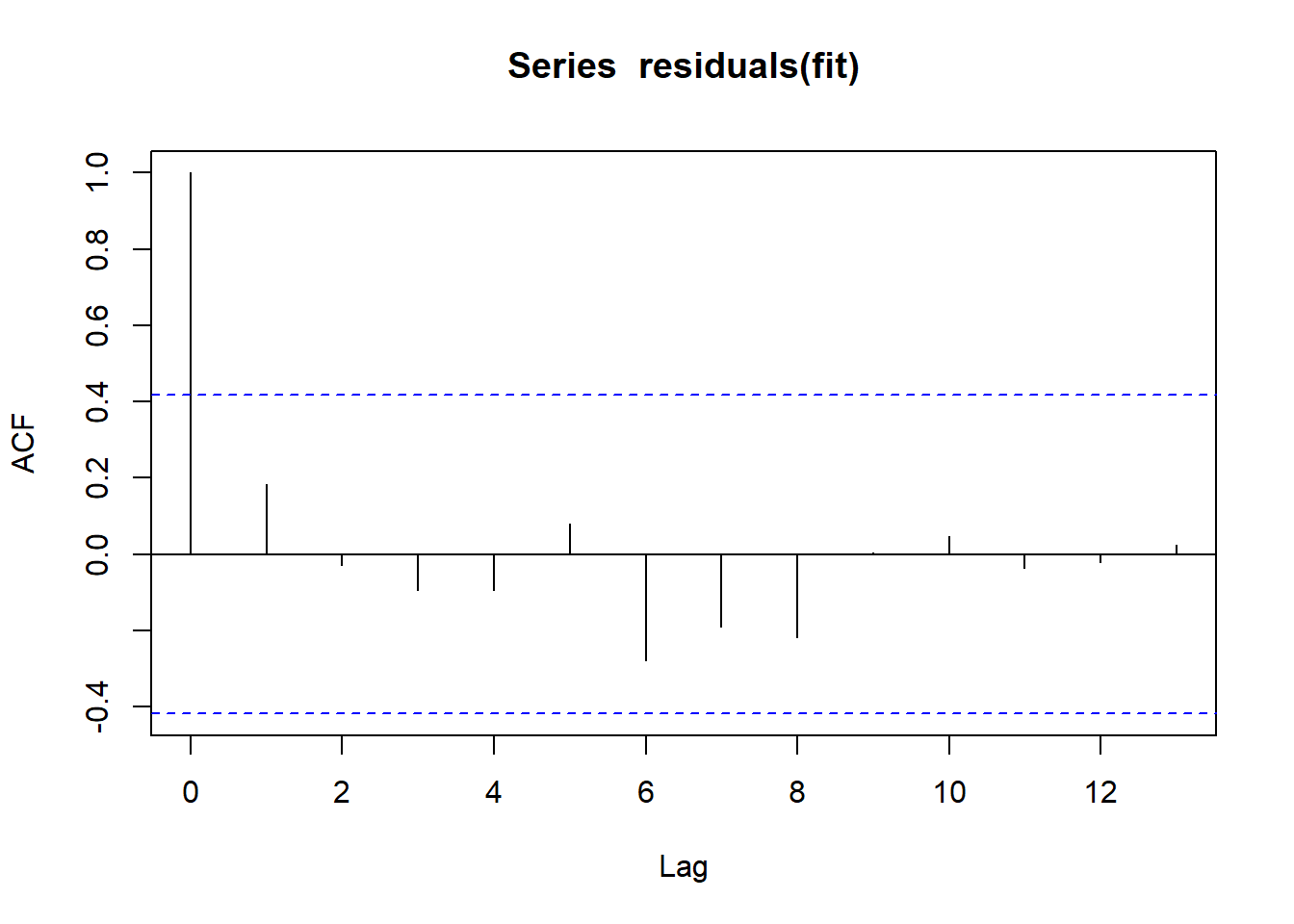
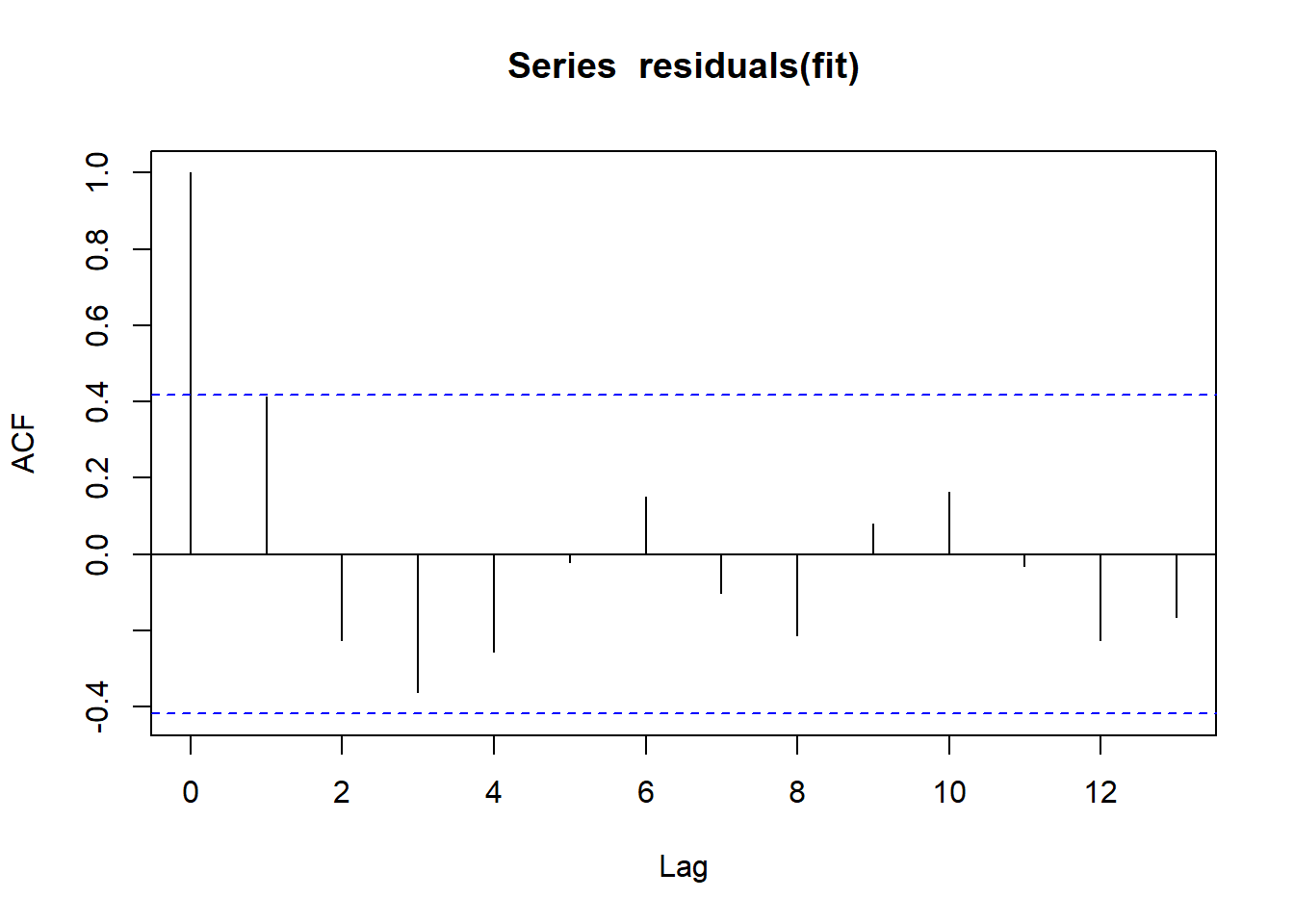
# independence
durbinWatsonTest(fit)
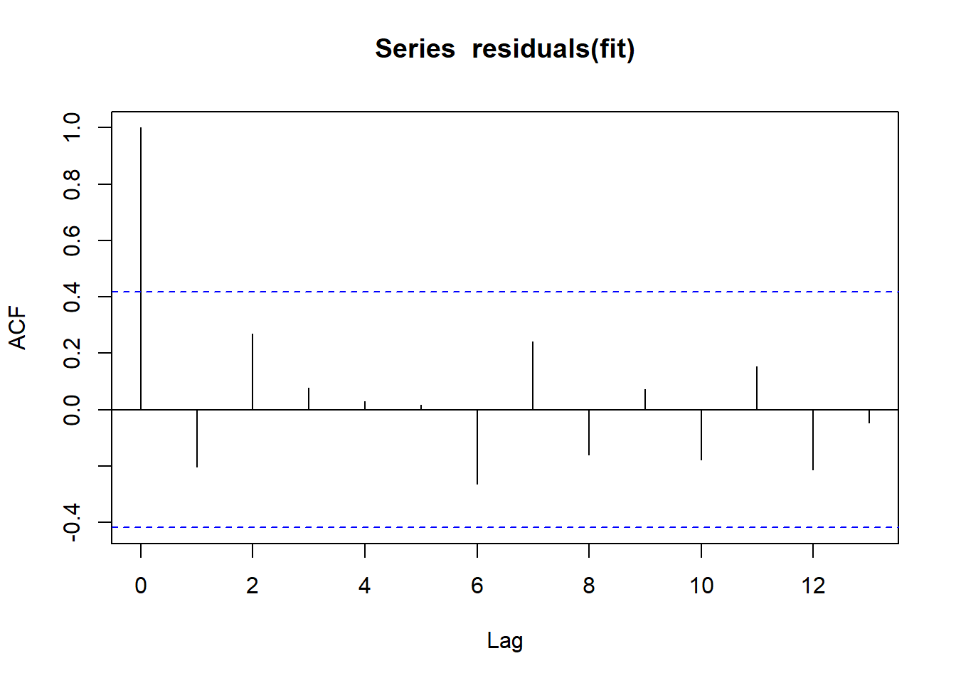
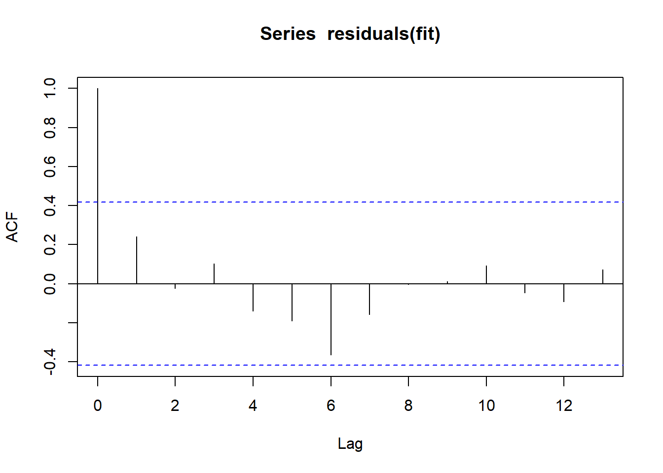
layout(matrix(c(1),1,1))
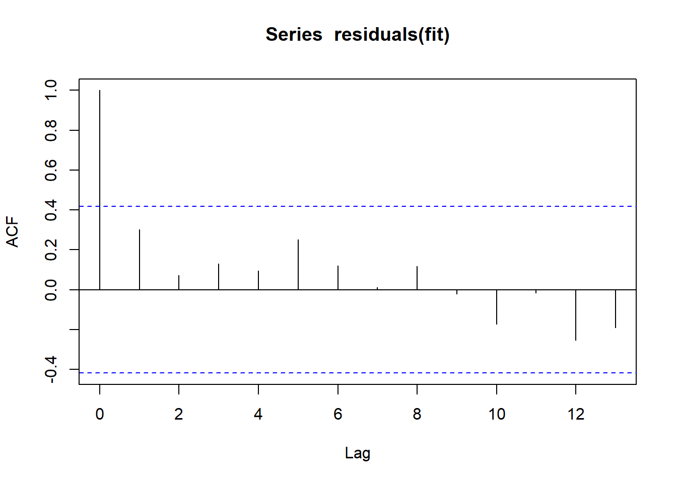
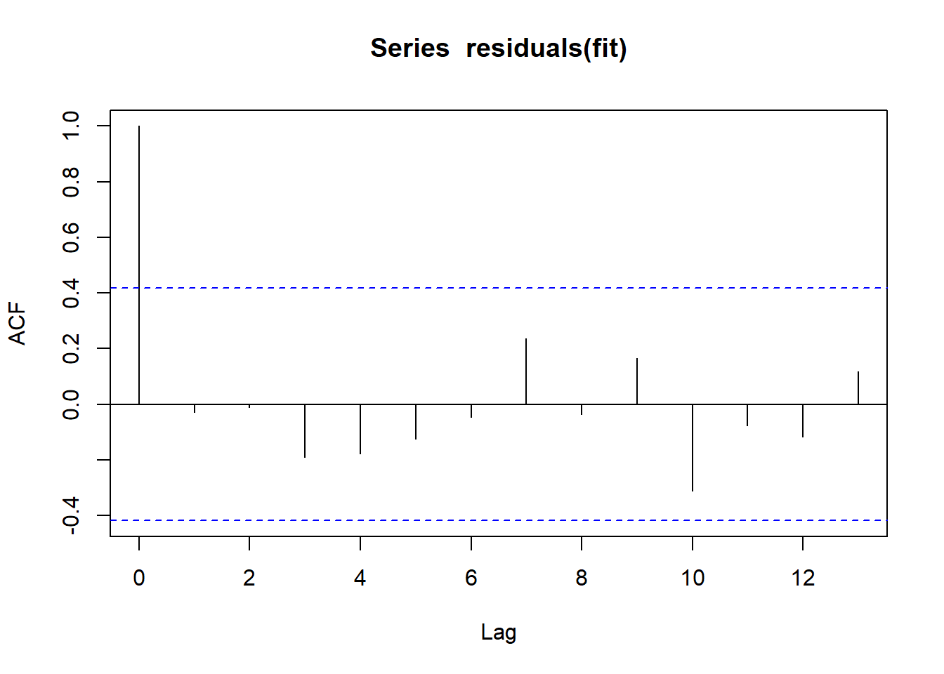
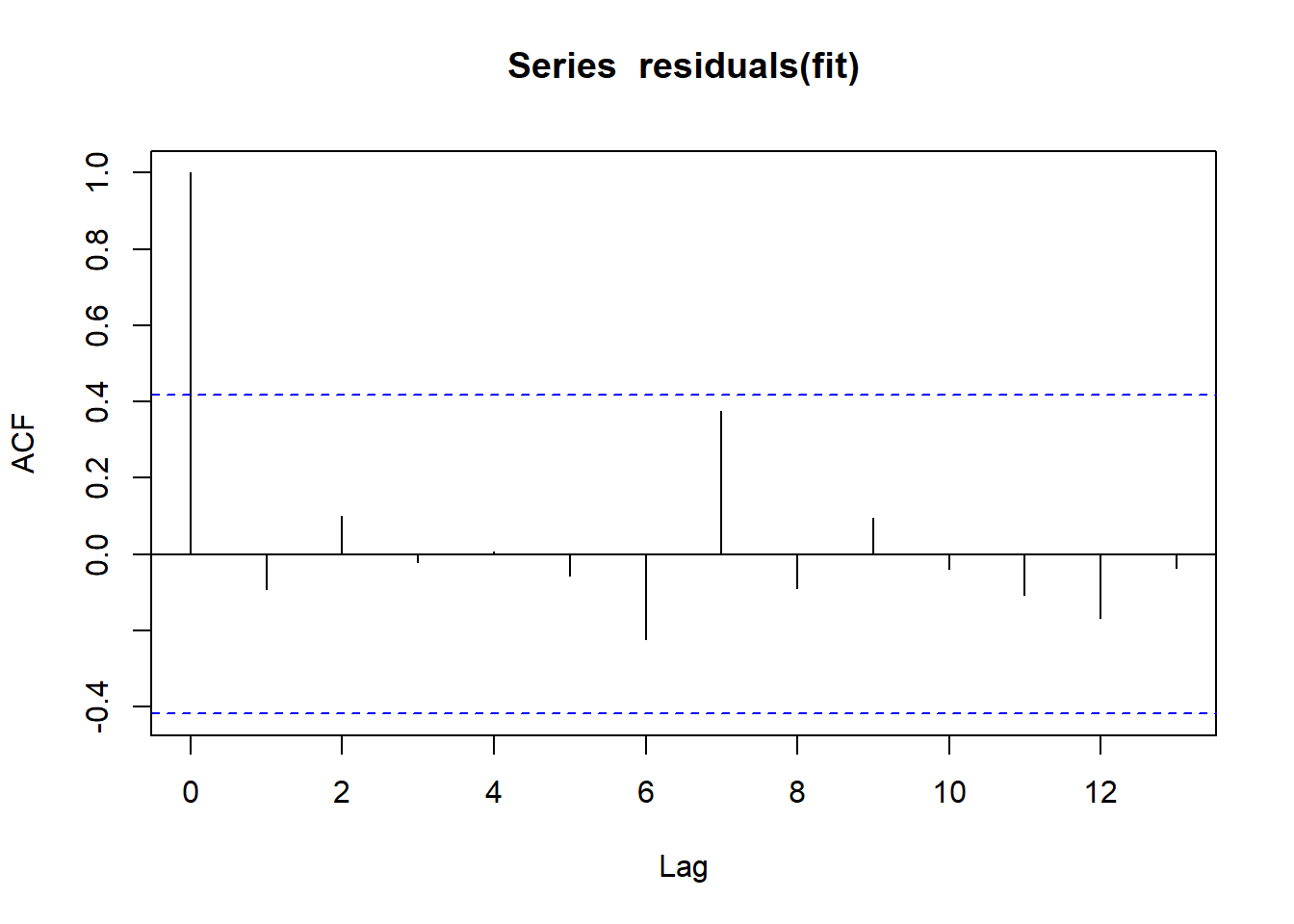
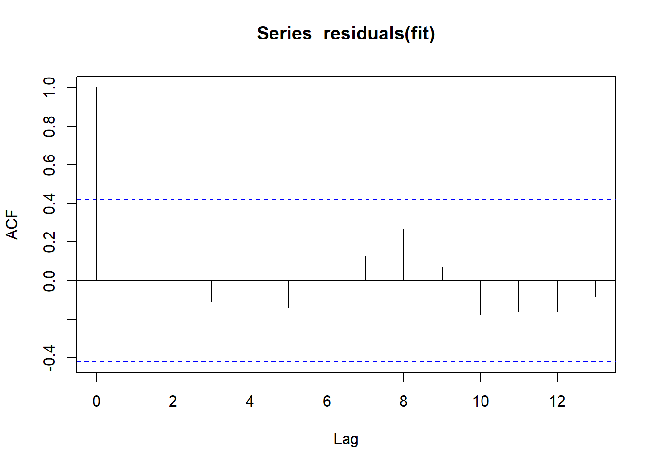
acf(residuals(fit))
# nice wrapper function to generally test a lot of stuff
gvmodel <- gvlma(fit)
summary(gvmodel)
}
=======================
=======================
Outcome:     Glucose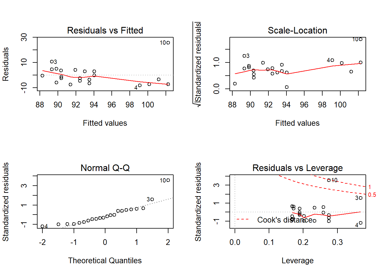
Call:
lm(formula = form, data = mydata)

Residuals:
   Min     1Q Median     3Q    Max
-8.113 -5.496 -1.866  3.483 25.742

Coefficients:
            Estimate Std. Error t value Pr(>|t|)
(Intercept)  93.0792     3.5046  26.559 2.78e-15 ***
IntB         -1.5742     5.2540  -0.300    0.768
Post         -3.6667     4.9115  -0.747    0.466
c.age        -0.5242     0.9690  -0.541    0.596
IntB:Post    13.4667     7.2850   1.849    0.082 .
---
Signif. codes:  0 '***' 0.001 '**' 0.01 '*' 0.05 '.' 0.1 ' ' 1

Residual standard error: 8.507 on 17 degrees of freedom
Multiple R-squared:  0.2532,    Adjusted R-squared:  0.07743
F-statistic: 1.441 on 4 and 17 DF,  p-value: 0.2636


ASSESSMENT OF THE LINEAR MODEL ASSUMPTIONS
USING THE GLOBAL TEST ON 4 DEGREES-OF-FREEDOM:
Level of Significance =  0.05

Call:
 gvlma(x = fit)

                     Value   p-value                   Decision
Global Stat        32.4590 1.541e-06 Assumptions NOT satisfied!
Skewness           11.5465 6.788e-04 Assumptions NOT satisfied!
Kurtosis           13.4942 2.393e-04 Assumptions NOT satisfied!
Link Function       7.1556 7.473e-03 Assumptions NOT satisfied!
Heteroscedasticity  0.2628 6.082e-01    Assumptions acceptable.


=======================
=======================
Outcome:     BUN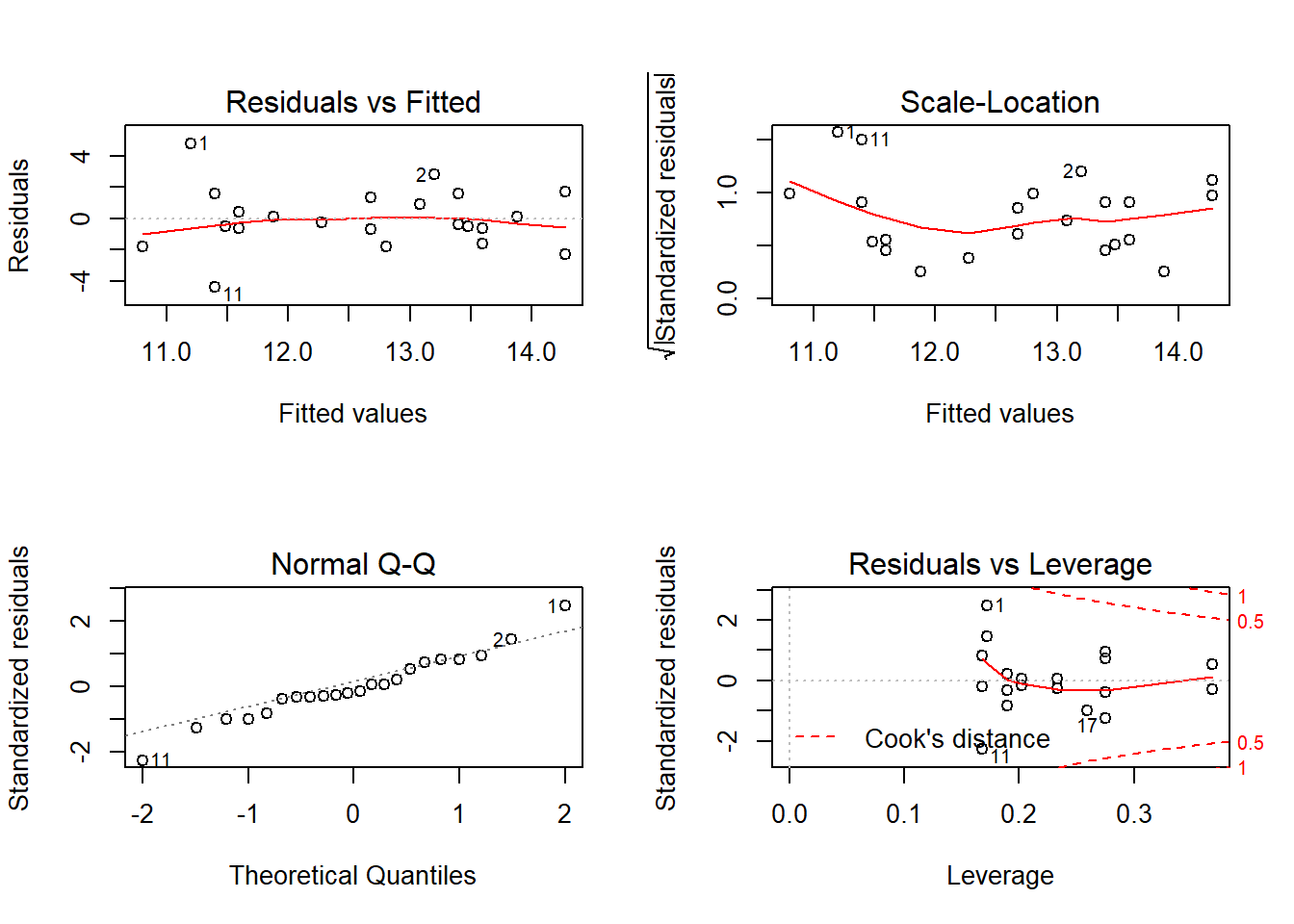

Call:
lm(formula = form, data = mydata)

Residuals:
    Min      1Q  Median      3Q     Max
-4.3997 -0.6578 -0.3396  1.2209  4.7993

Coefficients:
            Estimate Std. Error t value Pr(>|t|)
(Intercept)  11.2369     0.8780  12.798 3.73e-10 ***
IntB          2.6789     1.3162   2.035   0.0577 .
Post          2.0000     1.2305   1.625   0.1225
c.age        -0.1990     0.2428  -0.820   0.4238
IntB:Post    -3.6000     1.8251  -1.973   0.0650 .
---
Signif. codes:  0 '***' 0.001 '**' 0.01 '*' 0.05 '.' 0.1 ' ' 1

Residual standard error: 2.131 on 17 degrees of freedom
Multiple R-squared:  0.2362,    Adjusted R-squared:  0.05645
F-statistic: 1.314 on 4 and 17 DF,  p-value: 0.3045


ASSESSMENT OF THE LINEAR MODEL ASSUMPTIONS
USING THE GLOBAL TEST ON 4 DEGREES-OF-FREEDOM:
Level of Significance =  0.05

Call:
 gvlma(x = fit)

                    Value p-value                   Decision
Global Stat        6.1746 0.18648    Assumptions acceptable.
Skewness           0.2160 0.64214    Assumptions acceptable.
Kurtosis           0.6861 0.40748    Assumptions acceptable.
Link Function      0.2798 0.59686    Assumptions acceptable.
Heteroscedasticity 4.9928 0.02545 Assumptions NOT satisfied!


=======================
=======================
Outcome:     Creatinine
Call:
lm(formula = form, data = mydata)

Residuals:
      Min        1Q    Median        3Q       Max
-0.150164 -0.064169 -0.001211  0.062296  0.138817

Coefficients:
              Estimate Std. Error t value Pr(>|t|)
(Intercept)  0.7597609  0.0365006  20.815 1.56e-13 ***
IntB         0.0845260  0.0547198   1.545    0.141
Post         0.0750000  0.0511536   1.466    0.161
c.age       -0.0004931  0.0100926  -0.049    0.962
IntB:Post   -0.0690000  0.0758731  -0.909    0.376
---
Signif. codes:  0 '***' 0.001 '**' 0.01 '*' 0.05 '.' 0.1 ' ' 1

Residual standard error: 0.0886 on 17 degrees of freedom
Multiple R-squared:  0.1853,    Adjusted R-squared:  -0.00642
F-statistic: 0.9665 on 4 and 17 DF,  p-value: 0.4512


ASSESSMENT OF THE LINEAR MODEL ASSUMPTIONS
USING THE GLOBAL TEST ON 4 DEGREES-OF-FREEDOM:
Level of Significance =  0.05

Call:
 gvlma(x = fit)

                      Value p-value                Decision
Global Stat        0.786360  0.9403 Assumptions acceptable.
Skewness           0.001561  0.9685 Assumptions acceptable.
Kurtosis           0.595412  0.4403 Assumptions acceptable.
Link Function      0.163503  0.6860 Assumptions acceptable.
Heteroscedasticity 0.025885  0.8722 Assumptions acceptable.


=======================
=======================
Outcome:     Sodium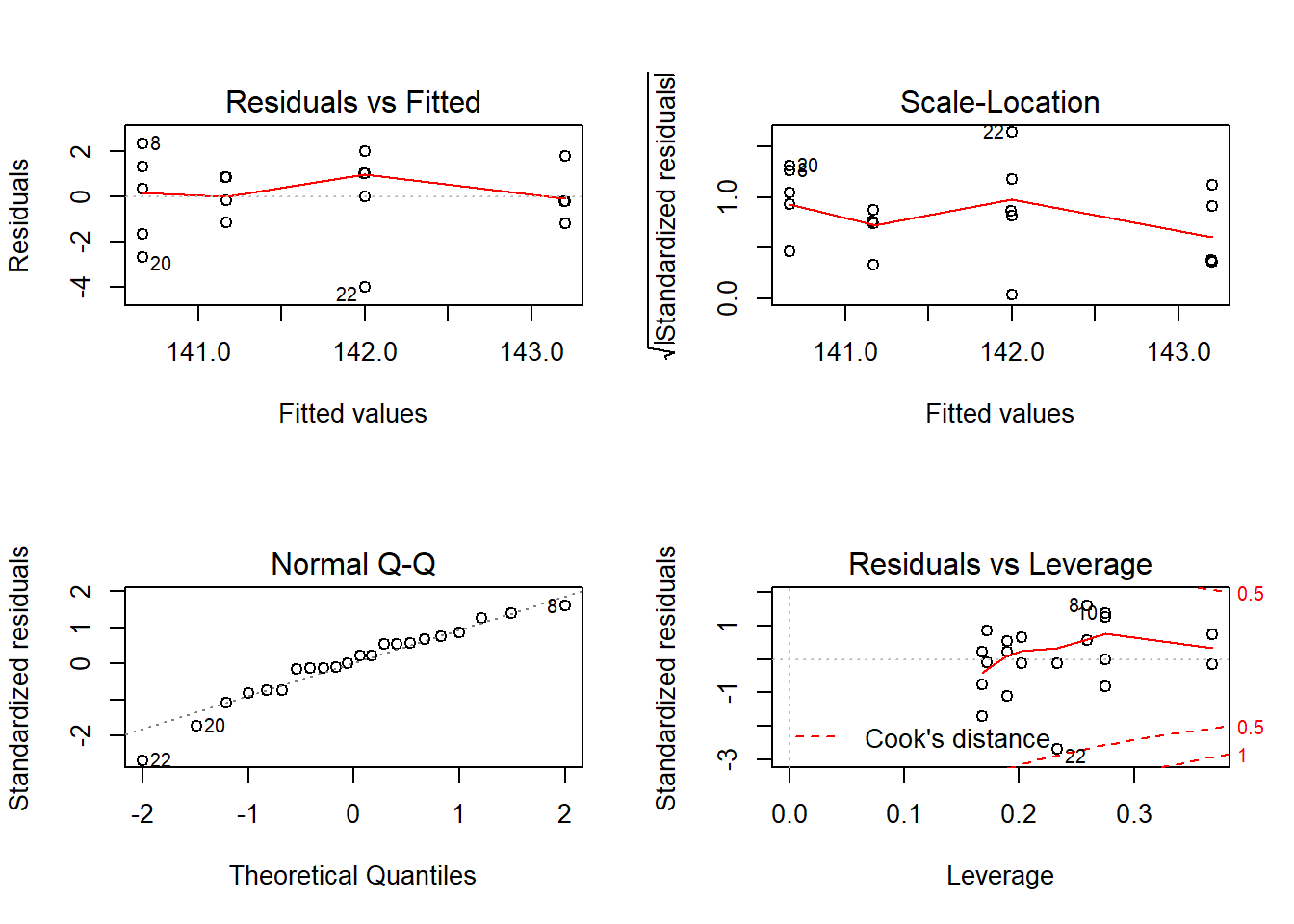

Call:
lm(formula = form, data = mydata)

Residuals:
    Min      1Q  Median      3Q     Max
-3.9986 -0.9253  0.1651  0.9587  2.3356

Coefficients:
              Estimate Std. Error t value Pr(>|t|)
(Intercept)  1.412e+02  6.992e-01 201.903   <2e-16 ***
IntB         2.034e+00  1.048e+00   1.941   0.0691 .
Post        -5.000e-01  9.799e-01  -0.510   0.6164
c.age       -8.651e-04  1.933e-01  -0.004   0.9965
IntB:Post   -7.000e-01  1.453e+00  -0.482   0.6362
---
Signif. codes:  0 '***' 0.001 '**' 0.01 '*' 0.05 '.' 0.1 ' ' 1

Residual standard error: 1.697 on 17 degrees of freedom
Multiple R-squared:  0.288, Adjusted R-squared:  0.1205
F-statistic: 1.719 on 4 and 17 DF,  p-value: 0.1922


ASSESSMENT OF THE LINEAR MODEL ASSUMPTIONS
USING THE GLOBAL TEST ON 4 DEGREES-OF-FREEDOM:
Level of Significance =  0.05

Call:
 gvlma(x = fit)

                    Value p-value                Decision
Global Stat        7.8333 0.09788 Assumptions acceptable.
Skewness           2.4541 0.11722 Assumptions acceptable.
Kurtosis           0.2386 0.62523 Assumptions acceptable.
Link Function      1.8066 0.17891 Assumptions acceptable.
Heteroscedasticity 3.3340 0.06786 Assumptions acceptable.


=======================
=======================
Outcome:     Potassium
Call:
lm(formula = form, data = mydata)

Residuals:
     Min       1Q   Median       3Q      Max
-0.47235 -0.26090 -0.02216  0.14516  1.06061

Coefficients:
            Estimate Std. Error t value Pr(>|t|)
(Intercept)  4.51750    0.16363  27.608 1.46e-15 ***
IntB        -0.07849    0.24531  -0.320    0.753
Post        -0.21667    0.22932  -0.945    0.358
c.age       -0.06704    0.04524  -1.482    0.157
IntB:Post    0.11667    0.34014   0.343    0.736
---
Signif. codes:  0 '***' 0.001 '**' 0.01 '*' 0.05 '.' 0.1 ' ' 1

Residual standard error: 0.3972 on 17 degrees of freedom
Multiple R-squared:  0.1722,    Adjusted R-squared:  -0.02253
F-statistic: 0.8843 on 4 and 17 DF,  p-value: 0.4941


ASSESSMENT OF THE LINEAR MODEL ASSUMPTIONS
USING THE GLOBAL TEST ON 4 DEGREES-OF-FREEDOM:
Level of Significance =  0.05

Call:
 gvlma(x = fit)

                     Value p-value                   Decision
Global Stat        7.43923 0.11442    Assumptions acceptable.
Skewness           4.45281 0.03484 Assumptions NOT satisfied!
Kurtosis           2.33163 0.12677    Assumptions acceptable.
Link Function      0.00619 0.93729    Assumptions acceptable.
Heteroscedasticity 0.64861 0.42061    Assumptions acceptable.


=======================
=======================
Outcome:     Chloride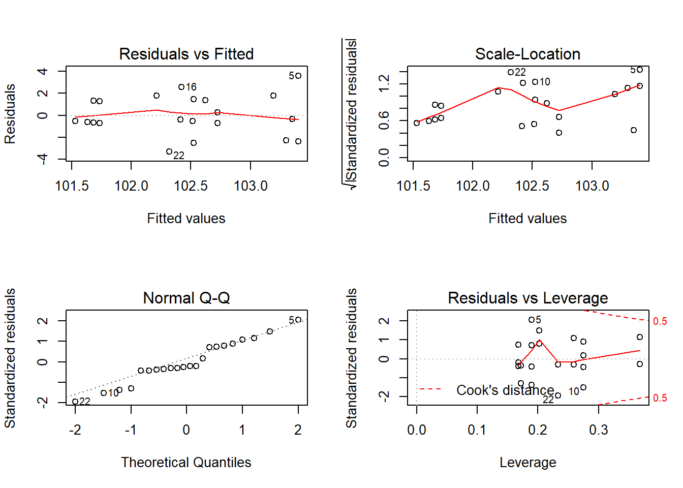

Call:
lm(formula = form, data = mydata)

Residuals:
    Min      1Q  Median      3Q     Max
-3.3170 -0.7144 -0.3819  1.3634  3.5975

Coefficients:
            Estimate Std. Error t value Pr(>|t|)
(Intercept) 103.3082     0.8047 128.384   <2e-16 ***
IntB         -0.6780     1.2063  -0.562    0.581
Post         -1.6667     1.1277  -1.478    0.158
c.age        -0.0519     0.2225  -0.233    0.818
IntB:Post     1.4667     1.6727   0.877    0.393
---
Signif. codes:  0 '***' 0.001 '**' 0.01 '*' 0.05 '.' 0.1 ' ' 1

Residual standard error: 1.953 on 17 degrees of freedom
Multiple R-squared:  0.1176,    Adjusted R-squared:  -0.09007
F-statistic: 0.5662 on 4 and 17 DF,  p-value: 0.6905


ASSESSMENT OF THE LINEAR MODEL ASSUMPTIONS
USING THE GLOBAL TEST ON 4 DEGREES-OF-FREEDOM:
Level of Significance =  0.05

Call:
 gvlma(x = fit)

                      Value p-value                Decision
Global Stat        0.497308  0.9738 Assumptions acceptable.
Skewness           0.007587  0.9306 Assumptions acceptable.
Kurtosis           0.266516  0.6057 Assumptions acceptable.
Link Function      0.207461  0.6488 Assumptions acceptable.
Heteroscedasticity 0.015744  0.9001 Assumptions acceptable.


=======================
=======================
Outcome:     Carbon_Dioxide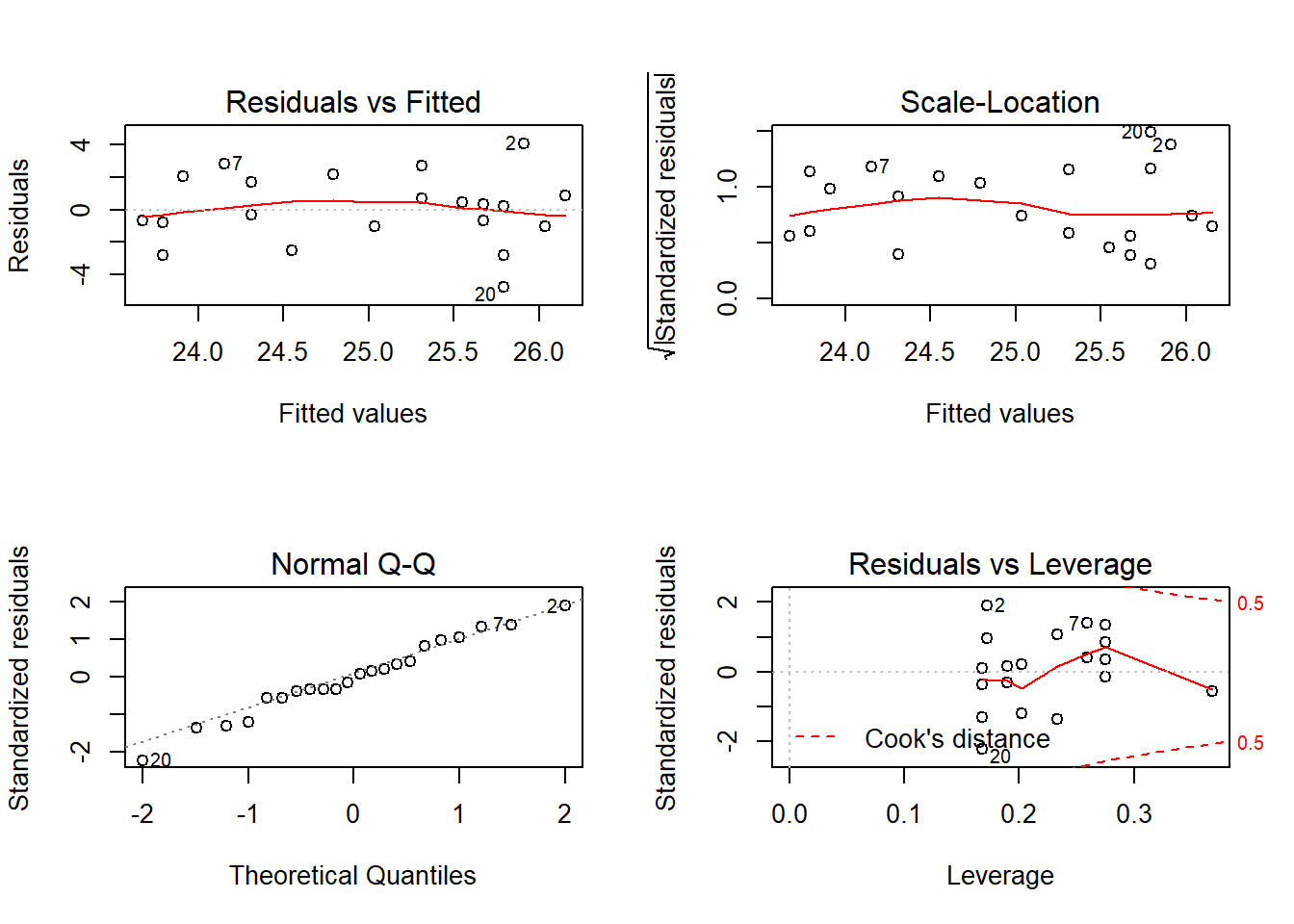

Call:
lm(formula = form, data = mydata)

Residuals:
    Min      1Q  Median      3Q     Max
-4.7933 -0.9730 -0.0523  1.4779  4.0865

Coefficients:
            Estimate Std. Error t value Pr(>|t|)
(Intercept)  23.8916     0.9736  24.539 1.03e-14 ***
IntB          0.6384     1.4596   0.437    0.667
Post          2.0000     1.3645   1.466    0.161
c.age         0.1202     0.2692   0.447    0.661
IntB:Post    -1.0000     2.0239  -0.494    0.628
---
Signif. codes:  0 '***' 0.001 '**' 0.01 '*' 0.05 '.' 0.1 ' ' 1

Residual standard error: 2.363 on 17 degrees of freedom
Multiple R-squared:  0.1442,    Adjusted R-squared:  -0.05714
F-statistic: 0.7162 on 4 and 17 DF,  p-value: 0.5923


ASSESSMENT OF THE LINEAR MODEL ASSUMPTIONS
USING THE GLOBAL TEST ON 4 DEGREES-OF-FREEDOM:
Level of Significance =  0.05

Call:
 gvlma(x = fit)

                     Value p-value                Decision
Global Stat        2.14800  0.7086 Assumptions acceptable.
Skewness           0.13256  0.7158 Assumptions acceptable.
Kurtosis           0.04022  0.8410 Assumptions acceptable.
Link Function      1.49279  0.2218 Assumptions acceptable.
Heteroscedasticity 0.48243  0.4873 Assumptions acceptable.


=======================
=======================
Outcome:     Calcium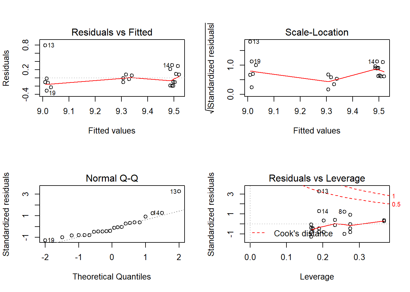
Call:
lm(formula = form, data = mydata)

Residuals:
     Min       1Q   Median       3Q      Max
-0.31482 -0.17012 -0.06351  0.08168  0.79072

Coefficients:
             Estimate Std. Error t value Pr(>|t|)
(Intercept)  9.019351   0.110992  81.261   <2e-16 ***
IntB         0.297428   0.166393   1.788   0.0917 .
Post         0.483333   0.155549   3.107   0.0064 **
c.age        0.005536   0.030690   0.180   0.8590
IntB:Post   -0.303333   0.230717  -1.315   0.2061
---
Signif. codes:  0 '***' 0.001 '**' 0.01 '*' 0.05 '.' 0.1 ' ' 1

Residual standard error: 0.2694 on 17 degrees of freedom
Multiple R-squared:  0.4244,    Adjusted R-squared:  0.2889
F-statistic: 3.133 on 4 and 17 DF,  p-value: 0.04214


ASSESSMENT OF THE LINEAR MODEL ASSUMPTIONS
USING THE GLOBAL TEST ON 4 DEGREES-OF-FREEDOM:
Level of Significance =  0.05

Call:
 gvlma(x = fit)

                     Value   p-value                   Decision
Global Stat        23.1065 0.0001206 Assumptions NOT satisfied!
Skewness            9.8606 0.0016885 Assumptions NOT satisfied!
Kurtosis            9.2705 0.0023288 Assumptions NOT satisfied!
Link Function       3.6266 0.0568615    Assumptions acceptable.
Heteroscedasticity  0.3488 0.5547935    Assumptions acceptable.


=======================
=======================
Outcome:     Cholesterol
Call:
lm(formula = form, data = mydata)

Residuals:
    Min      1Q  Median      3Q     Max
-60.985 -20.503  -3.721  24.219  51.534

Coefficients:
            Estimate Std. Error t value Pr(>|t|)
(Intercept)  154.723     14.902  10.383  8.9e-09 ***
IntB          46.010     22.340   2.060   0.0551 .
Post          10.667     20.884   0.511   0.6161
c.age         -1.260      4.120  -0.306   0.7636
IntB:Post     -2.467     30.976  -0.080   0.9375
---
Signif. codes:  0 '***' 0.001 '**' 0.01 '*' 0.05 '.' 0.1 ' ' 1

Residual standard error: 36.17 on 17 degrees of freedom
Multiple R-squared:  0.3293,    Adjusted R-squared:  0.1715
F-statistic: 2.087 on 4 and 17 DF,  p-value: 0.1274


ASSESSMENT OF THE LINEAR MODEL ASSUMPTIONS
USING THE GLOBAL TEST ON 4 DEGREES-OF-FREEDOM:
Level of Significance =  0.05

Call:
 gvlma(x = fit)

                     Value p-value                Decision
Global Stat        2.70701  0.6080 Assumptions acceptable.
Skewness           0.01125  0.9155 Assumptions acceptable.
Kurtosis           0.70279  0.4018 Assumptions acceptable.
Link Function      1.33685  0.2476 Assumptions acceptable.
Heteroscedasticity 0.65612  0.4179 Assumptions acceptable.


=======================
=======================
Outcome:     Triglycerides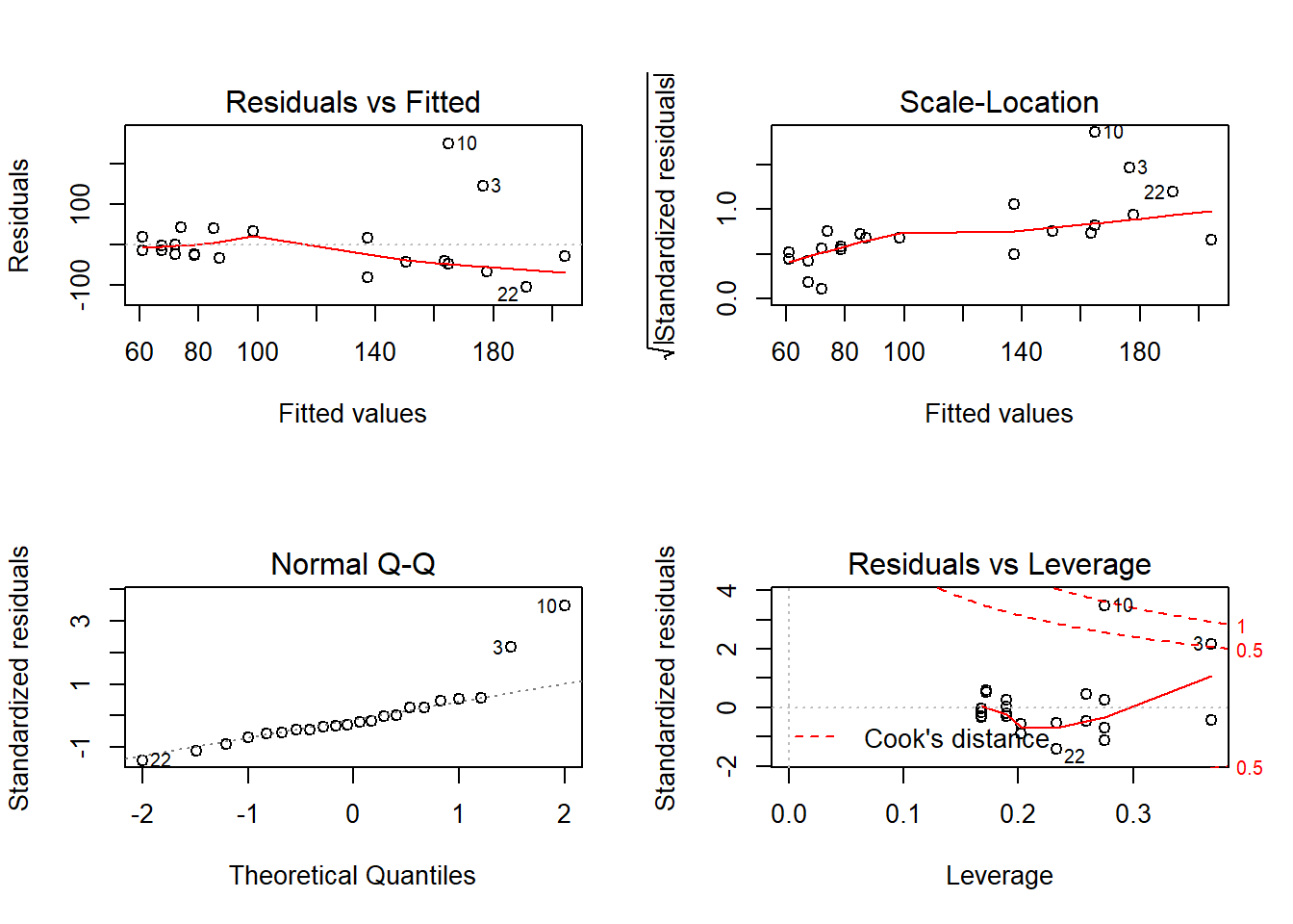

Call:
lm(formula = form, data = mydata)

Residuals:
    Min      1Q  Median      3Q     Max
-105.12  -37.94  -19.27   19.52  250.18

Coefficients:
            Estimate Std. Error t value Pr(>|t|)
(Intercept)   84.022     34.769   2.417   0.0272 *
IntB          65.152     52.124   1.250   0.2283
Post         -11.167     48.727  -0.229   0.8215
c.age          6.576      9.614   0.684   0.5032
IntB:Post     38.767     72.274   0.536   0.5986
---
Signif. codes:  0 '***' 0.001 '**' 0.01 '*' 0.05 '.' 0.1 ' ' 1

Residual standard error: 84.4 on 17 degrees of freedom
Multiple R-squared:  0.2977,    Adjusted R-squared:  0.1324
F-statistic: 1.801 on 4 and 17 DF,  p-value: 0.1751


ASSESSMENT OF THE LINEAR MODEL ASSUMPTIONS
USING THE GLOBAL TEST ON 4 DEGREES-OF-FREEDOM:
Level of Significance =  0.05

Call:
 gvlma(x = fit)

                     Value   p-value                   Decision
Global Stat        26.8974 2.085e-05 Assumptions NOT satisfied!
Skewness           12.4843 4.104e-04 Assumptions NOT satisfied!
Kurtosis           13.6347 2.220e-04 Assumptions NOT satisfied!
Link Function       0.5387 4.630e-01    Assumptions acceptable.
Heteroscedasticity  0.2397 6.244e-01    Assumptions acceptable.


=======================
=======================
Outcome:     HDL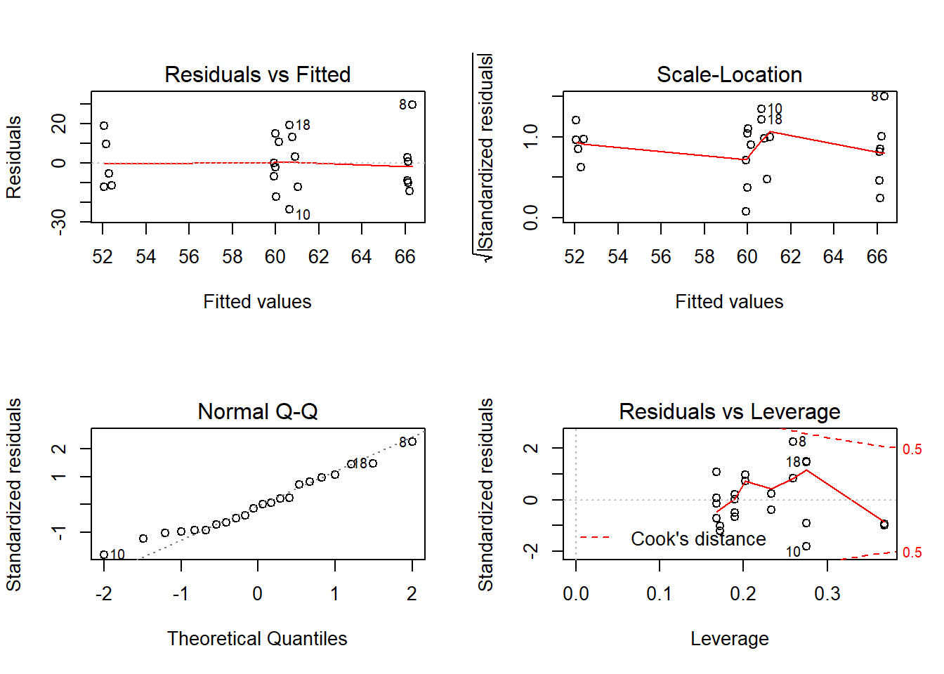

Call:
lm(formula = form, data = mydata)

Residuals:
     Min       1Q   Median       3Q      Max
-23.6547 -11.1001  -0.9495  10.5849  29.6719

Coefficients:
            Estimate Std. Error t value Pr(>|t|)
(Intercept) 60.02936    6.30676   9.518 3.18e-08 ***
IntB        -7.86459    9.45477  -0.832    0.417
Post         6.16667    8.83859   0.698    0.495
c.age        0.06055    1.74385   0.035    0.973
IntB:Post    2.43333   13.10974   0.186    0.855
---
Signif. codes:  0 '***' 0.001 '**' 0.01 '*' 0.05 '.' 0.1 ' ' 1

Residual standard error: 15.31 on 17 degrees of freedom
Multiple R-squared:  0.1185,    Adjusted R-squared:  -0.08889
F-statistic: 0.5714 on 4 and 17 DF,  p-value: 0.687


ASSESSMENT OF THE LINEAR MODEL ASSUMPTIONS
USING THE GLOBAL TEST ON 4 DEGREES-OF-FREEDOM:
Level of Significance =  0.05

Call:
 gvlma(x = fit)

                    Value p-value                Decision
Global Stat        4.3646  0.3589 Assumptions acceptable.
Skewness           0.5017  0.4788 Assumptions acceptable.
Kurtosis           0.4370  0.5086 Assumptions acceptable.
Link Function      2.9838  0.0841 Assumptions acceptable.
Heteroscedasticity 0.4422  0.5061 Assumptions acceptable.


=======================
=======================
Outcome:     LDL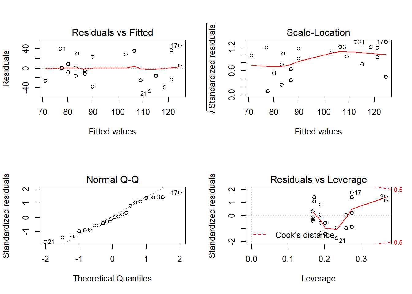

Call:
lm(formula = form, data = mydata)

Residuals:
    Min      1Q  Median      3Q     Max
-47.561 -21.674  -1.805  26.744  46.341

Coefficients:
            Estimate Std. Error t value Pr(>|t|)
(Intercept)   77.700     12.858   6.043 1.32e-05 ***
IntB          41.459     19.276   2.151   0.0462 *
Post           6.667     18.019   0.370   0.7160
c.age         -3.024      3.555  -0.851   0.4068
IntB:Post    -10.127     26.727  -0.379   0.7095
---
Signif. codes:  0 '***' 0.001 '**' 0.01 '*' 0.05 '.' 0.1 ' ' 1

Residual standard error: 31.21 on 17 degrees of freedom
Multiple R-squared:  0.2932,    Adjusted R-squared:  0.1269
F-statistic: 1.763 on 4 and 17 DF,  p-value: 0.1829


ASSESSMENT OF THE LINEAR MODEL ASSUMPTIONS
USING THE GLOBAL TEST ON 4 DEGREES-OF-FREEDOM:
Level of Significance =  0.05

Call:
 gvlma(x = fit)

                      Value p-value                Decision
Global Stat        1.447064  0.8360 Assumptions acceptable.
Skewness           0.026420  0.8709 Assumptions acceptable.
Kurtosis           1.180484  0.2773 Assumptions acceptable.
Link Function      0.236073  0.6271 Assumptions acceptable.
Heteroscedasticity 0.004087  0.9490 Assumptions acceptable.


=======================
=======================
Outcome:     LDL_HDL_Ratio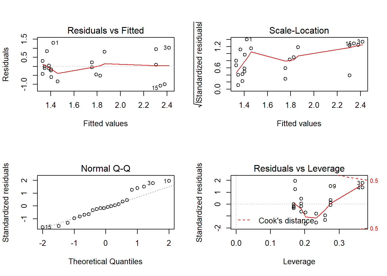
Call:
lm(formula = form, data = mydata)

Residuals:
     Min       1Q   Median       3Q      Max
-1.07463 -0.44308 -0.08132  0.27873  1.29772

Coefficients:
            Estimate Std. Error t value Pr(>|t|)
(Intercept)  1.41893    0.30068   4.719 0.000198 ***
IntB         0.92235    0.45076   2.046 0.056528 .
Post        -0.05500    0.42139  -0.131 0.897686
c.age        0.01843    0.08314   0.222 0.827249
IntB:Post   -0.49900    0.62502  -0.798 0.435664
---
Signif. codes:  0 '***' 0.001 '**' 0.01 '*' 0.05 '.' 0.1 ' ' 1

Residual standard error: 0.7299 on 17 degrees of freedom
Multiple R-squared:  0.274, Adjusted R-squared:  0.1032
F-statistic: 1.604 on 4 and 17 DF,  p-value: 0.2189


ASSESSMENT OF THE LINEAR MODEL ASSUMPTIONS
USING THE GLOBAL TEST ON 4 DEGREES-OF-FREEDOM:
Level of Significance =  0.05

Call:
 gvlma(x = fit)

                    Value p-value                Decision
Global Stat        3.5627  0.4684 Assumptions acceptable.
Skewness           0.4087  0.5226 Assumptions acceptable.
Kurtosis           0.4020  0.5260 Assumptions acceptable.
Link Function      0.2042  0.6514 Assumptions acceptable.
Heteroscedasticity 2.5478  0.1104 Assumptions acceptable.


=======================
=======================
Outcome:     hsCRP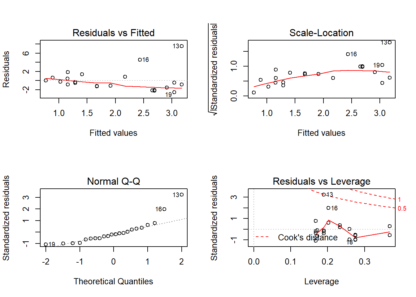
Call:
lm(formula = form, data = mydata)

Residuals:
    Min      1Q  Median      3Q     Max
-2.5433 -1.2468 -0.4666  0.5678  7.5268

Coefficients:
            Estimate Std. Error t value Pr(>|t|)
(Intercept)   2.9370     1.0620   2.766   0.0132 *
IntB         -1.5014     1.5921  -0.943   0.3589
Post         -1.8833     1.4883  -1.265   0.2228
c.age        -0.1299     0.2936  -0.442   0.6637
IntB:Post     2.9033     2.2075   1.315   0.2059
---
Signif. codes:  0 '***' 0.001 '**' 0.01 '*' 0.05 '.' 0.1 ' ' 1

Residual standard error: 2.578 on 17 degrees of freedom
Multiple R-squared:  0.1154,    Adjusted R-squared:  -0.09275
F-statistic: 0.5544 on 4 and 17 DF,  p-value: 0.6986


ASSESSMENT OF THE LINEAR MODEL ASSUMPTIONS
USING THE GLOBAL TEST ON 4 DEGREES-OF-FREEDOM:
Level of Significance =  0.05

Call:
 gvlma(x = fit)

                     Value   p-value                   Decision
Global Stat        26.2310 2.843e-05 Assumptions NOT satisfied!
Skewness           12.6428 3.770e-04 Assumptions NOT satisfied!
Kurtosis           11.3214 7.662e-04 Assumptions NOT satisfied!
Link Function       1.2733 2.591e-01    Assumptions acceptable.
Heteroscedasticity  0.9934 3.189e-01    Assumptions acceptable.


=======================
=======================
Outcome:     Insulin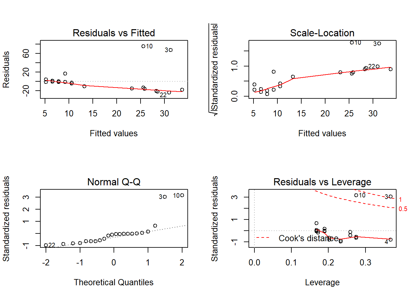
Call:
lm(formula = form, data = mydata)

Residuals:
    Min      1Q  Median      3Q     Max
-23.965 -15.153  -1.912  -0.034  75.447

Coefficients:
            Estimate Std. Error t value Pr(>|t|)
(Intercept)   7.6560    11.5542   0.663    0.516
IntB         17.9569    17.3215   1.037    0.314
Post          2.6667    16.1926   0.165    0.871
c.age         1.3529     3.1948   0.423    0.677
IntB:Post    -0.2667    24.0176  -0.011    0.991

Residual standard error: 28.05 on 17 degrees of freedom
Multiple R-squared:  0.1414,    Adjusted R-squared:  -0.06067
F-statistic: 0.6997 on 4 and 17 DF,  p-value: 0.6027


ASSESSMENT OF THE LINEAR MODEL ASSUMPTIONS
USING THE GLOBAL TEST ON 4 DEGREES-OF-FREEDOM:
Level of Significance =  0.05

Call:
 gvlma(x = fit)

                    Value   p-value                   Decision
Global Stat        30.834 3.310e-06 Assumptions NOT satisfied!
Skewness           16.186 5.741e-05 Assumptions NOT satisfied!
Kurtosis           12.626 3.803e-04 Assumptions NOT satisfied!
Link Function       0.112 7.378e-01    Assumptions acceptable.
Heteroscedasticity  1.909 1.671e-01    Assumptions acceptable.


=======================
=======================
Outcome:     PYY
Call:
lm(formula = form, data = mydata)

Residuals:
    Min      1Q  Median      3Q     Max
-142.85  -89.12  -41.44  -14.65  581.35

Coefficients:
            Estimate Std. Error t value Pr(>|t|)
(Intercept)  160.501     77.397   2.074   0.0536 .
IntB        -103.935    116.029  -0.896   0.3829
Post         -32.087    108.467  -0.296   0.7710
c.age          5.795     21.401   0.271   0.7898
IntB:Post     26.901    160.883   0.167   0.8692
---
Signif. codes:  0 '***' 0.001 '**' 0.01 '*' 0.05 '.' 0.1 ' ' 1

Residual standard error: 187.9 on 17 degrees of freedom
Multiple R-squared:  0.06906,   Adjusted R-squared:  -0.15
F-statistic: 0.3153 on 4 and 17 DF,  p-value: 0.8638


ASSESSMENT OF THE LINEAR MODEL ASSUMPTIONS
USING THE GLOBAL TEST ON 4 DEGREES-OF-FREEDOM:
Level of Significance =  0.05

Call:
 gvlma(x = fit)

                    Value   p-value                   Decision
Global Stat        63.837 4.522e-13 Assumptions NOT satisfied!
Skewness           20.571 5.747e-06 Assumptions NOT satisfied!
Kurtosis           23.973 9.772e-07 Assumptions NOT satisfied!
Link Function       1.146 2.845e-01    Assumptions acceptable.
Heteroscedasticity 18.148 2.043e-05 Assumptions NOT satisfied!
Results Adjusted for Multiple Comparisons
all_results <- unlist.res(results.out)Joining, by = c("Estimate", "Std. Error", "t value", "Pr(>|t|)", "Outcome", "Parameter")
Joining, by = c("Estimate", "Std. Error", "t value", "Pr(>|t|)", "Outcome", "Parameter")
Joining, by = c("Estimate", "Std. Error", "t value", "Pr(>|t|)", "Outcome", "Parameter")
Joining, by = c("Estimate", "Std. Error", "t value", "Pr(>|t|)", "Outcome", "Parameter")
Joining, by = c("Estimate", "Std. Error", "t value", "Pr(>|t|)", "Outcome", "Parameter")
Joining, by = c("Estimate", "Std. Error", "t value", "Pr(>|t|)", "Outcome", "Parameter")
Joining, by = c("Estimate", "Std. Error", "t value", "Pr(>|t|)", "Outcome", "Parameter")
Joining, by = c("Estimate", "Std. Error", "t value", "Pr(>|t|)", "Outcome", "Parameter")
Joining, by = c("Estimate", "Std. Error", "t value", "Pr(>|t|)", "Outcome", "Parameter")
Joining, by = c("Estimate", "Std. Error", "t value", "Pr(>|t|)", "Outcome", "Parameter")
Joining, by = c("Estimate", "Std. Error", "t value", "Pr(>|t|)", "Outcome", "Parameter")
Joining, by = c("Estimate", "Std. Error", "t value", "Pr(>|t|)", "Outcome", "Parameter")
Joining, by = c("Estimate", "Std. Error", "t value", "Pr(>|t|)", "Outcome", "Parameter")
Joining, by = c("Estimate", "Std. Error", "t value", "Pr(>|t|)", "Outcome", "Parameter")
Joining, by = c("Estimate", "Std. Error", "t value", "Pr(>|t|)", "Outcome", "Parameter")all_results <- filter(all_results, Parameter %in% c("IntB", "Post", "IntB:Post"))
all_results$p.adj <- p.adjust(all_results$`Pr(>|t|)`, "fdr")
all_results$sigflag <- ifelse(all_results$p.adj < 0.05, "*", " ")
all_results$`Pr(>|t|)` <- round(all_results$`Pr(>|t|)`, 3)
all_results$p.adj.fdr <- round(all_results$p.adj, 3)
all_results <- all_results[, c(5:6, 1:4, 7:8)]
kable(all_results, format="html", digits=3) %>%
kable_styling(full_width = T)| Outcome | Parameter | Estimate | Std. Error | t value | Pr(>|t|) | p.adj | sigflag |
|---|---|---|---|---|---|---|---|
| Glucose | IntB | -1.574 | 5.254 | -0.300 | 0.768 | 0.903 | |
| Glucose | Post | -3.667 | 4.912 | -0.747 | 0.466 | 0.828 | |
| Glucose | IntB:Post | 13.467 | 7.285 | 1.849 | 0.082 | 0.489 | |
| BUN | IntB | 2.679 | 1.316 | 2.035 | 0.058 | 0.474 | |
| BUN | Post | 2.000 | 1.230 | 1.625 | 0.122 | 0.552 | |
| BUN | IntB:Post | -3.600 | 1.825 | -1.973 | 0.065 | 0.474 | |
| Creatinine | IntB | 0.085 | 0.055 | 1.545 | 0.141 | 0.552 | |
| Creatinine | Post | 0.075 | 0.051 | 1.466 | 0.161 | 0.552 | |
| Creatinine | IntB:Post | -0.069 | 0.076 | -0.909 | 0.376 | 0.786 | |
| Sodium | IntB | 2.034 | 1.048 | 1.941 | 0.069 | 0.474 | |
| Sodium | Post | -0.500 | 0.980 | -0.510 | 0.616 | 0.898 | |
| Sodium | IntB:Post | -0.700 | 1.453 | -0.482 | 0.636 | 0.898 | |
| Potassium | IntB | -0.078 | 0.245 | -0.320 | 0.753 | 0.903 | |
| Potassium | Post | -0.217 | 0.229 | -0.945 | 0.358 | 0.786 | |
| Potassium | IntB:Post | 0.117 | 0.340 | 0.343 | 0.736 | 0.903 | |
| Chloride | IntB | -0.678 | 1.206 | -0.562 | 0.581 | 0.898 | |
| Chloride | Post | -1.667 | 1.128 | -1.478 | 0.158 | 0.552 | |
| Chloride | IntB:Post | 1.467 | 1.673 | 0.877 | 0.393 | 0.786 | |
| Carbon_Dioxide | IntB | 0.638 | 1.460 | 0.437 | 0.667 | 0.903 | |
| Carbon_Dioxide | Post | 2.000 | 1.364 | 1.466 | 0.161 | 0.552 | |
| Carbon_Dioxide | IntB:Post | -1.000 | 2.024 | -0.494 | 0.628 | 0.898 | |
| Calcium | IntB | 0.297 | 0.166 | 1.788 | 0.092 | 0.489 | |
| Calcium | Post | 0.483 | 0.156 | 3.107 | 0.006 | 0.307 | |
| Calcium | IntB:Post | -0.303 | 0.231 | -1.315 | 0.206 | 0.609 | |
| Cholesterol | IntB | 46.010 | 22.340 | 2.060 | 0.055 | 0.474 | |
| Cholesterol | Post | 10.667 | 20.884 | 0.511 | 0.616 | 0.898 | |
| Cholesterol | IntB:Post | -2.467 | 30.976 | -0.080 | 0.937 | 0.957 | |
| Triglycerides | IntB | 65.152 | 52.124 | 1.250 | 0.228 | 0.609 | |
| Triglycerides | Post | -11.167 | 48.727 | -0.229 | 0.821 | 0.929 | |
| Triglycerides | IntB:Post | 38.767 | 72.274 | 0.536 | 0.599 | 0.898 | |
| HDL | IntB | -7.865 | 9.455 | -0.832 | 0.417 | 0.801 | |
| HDL | Post | 6.167 | 8.839 | 0.698 | 0.495 | 0.848 | |
| HDL | IntB:Post | 2.433 | 13.110 | 0.186 | 0.855 | 0.929 | |
| LDL | IntB | 41.459 | 19.276 | 2.151 | 0.046 | 0.474 | |
| LDL | Post | 6.667 | 18.019 | 0.370 | 0.716 | 0.903 | |
| LDL | IntB:Post | -10.127 | 26.727 | -0.379 | 0.709 | 0.903 | |
| LDL_HDL_Ratio | IntB | 0.922 | 0.451 | 2.046 | 0.057 | 0.474 | |
| LDL_HDL_Ratio | Post | -0.055 | 0.421 | -0.131 | 0.898 | 0.937 | |
| LDL_HDL_Ratio | IntB:Post | -0.499 | 0.625 | -0.798 | 0.436 | 0.804 | |
| hsCRP | IntB | -1.501 | 1.592 | -0.943 | 0.359 | 0.786 | |
| hsCRP | Post | -1.883 | 1.488 | -1.265 | 0.223 | 0.609 | |
| hsCRP | IntB:Post | 2.903 | 2.208 | 1.315 | 0.206 | 0.609 | |
| Insulin | IntB | 17.957 | 17.322 | 1.037 | 0.314 | 0.786 | |
| Insulin | Post | 2.667 | 16.193 | 0.165 | 0.871 | 0.929 | |
| Insulin | IntB:Post | -0.267 | 24.018 | -0.011 | 0.991 | 0.991 | |
| PYY | IntB | -103.935 | 116.029 | -0.896 | 0.383 | 0.786 | |
| PYY | Post | -32.087 | 108.467 | -0.296 | 0.771 | 0.903 | |
| PYY | IntB:Post | 26.901 | 160.883 | 0.167 | 0.869 | 0.929 |
#readr::write_csv(all_results, "tab/results_blood_data.csv")
sessionInfo()R version 3.6.3 (2020-02-29)
Platform: x86_64-w64-mingw32/x64 (64-bit)
Running under: Windows 10 x64 (build 18362)
Matrix products: default
locale:
[1] LC_COLLATE=English_United States.1252
[2] LC_CTYPE=English_United States.1252
[3] LC_MONETARY=English_United States.1252
[4] LC_NUMERIC=C
[5] LC_TIME=English_United States.1252
attached base packages:
[1] stats graphics grDevices utils datasets methods base
other attached packages:
[1] cowplot_1.0.0 microbiome_1.8.0 car_3.0-8 carData_3.0-4
[5] gvlma_1.0.0.3 patchwork_1.0.0 viridis_0.5.1 viridisLite_0.3.0
[9] gridExtra_2.3 xtable_1.8-4 kableExtra_1.1.0 plyr_1.8.6
[13] data.table_1.12.8 readxl_1.3.1 forcats_0.5.0 stringr_1.4.0
[17] dplyr_0.8.5 purrr_0.3.4 readr_1.3.1 tidyr_1.1.0
[21] tibble_3.0.1 ggplot2_3.3.0 tidyverse_1.3.0 lmerTest_3.1-2
[25] lme4_1.1-23 Matrix_1.2-18 vegan_2.5-6 lattice_0.20-38
[29] permute_0.9-5 phyloseq_1.30.0
loaded via a namespace (and not attached):
[1] Rtsne_0.15 minqa_1.2.4 colorspace_1.4-1
[4] rio_0.5.16 ellipsis_0.3.1 rprojroot_1.3-2
[7] XVector_0.26.0 fs_1.4.1 rstudioapi_0.11
[10] farver_2.0.3 fansi_0.4.1 lubridate_1.7.8
[13] xml2_1.3.2 codetools_0.2-16 splines_3.6.3
[16] knitr_1.28 ade4_1.7-15 jsonlite_1.6.1
[19] workflowr_1.6.2 nloptr_1.2.2.1 broom_0.5.6
[22] cluster_2.1.0 dbplyr_1.4.4 BiocManager_1.30.10
[25] compiler_3.6.3 httr_1.4.1 backports_1.1.7
[28] assertthat_0.2.1 cli_2.0.2 later_1.0.0
[31] htmltools_0.4.0 tools_3.6.3 igraph_1.2.5
[34] gtable_0.3.0 glue_1.4.1 reshape2_1.4.4
[37] Rcpp_1.0.4.6 Biobase_2.46.0 cellranger_1.1.0
[40] vctrs_0.3.0 Biostrings_2.54.0 multtest_2.42.0
[43] ape_5.3 nlme_3.1-144 iterators_1.0.12
[46] xfun_0.14 openxlsx_4.1.5 rvest_0.3.5
[49] lifecycle_0.2.0 statmod_1.4.34 zlibbioc_1.32.0
[52] MASS_7.3-51.5 scales_1.1.1 hms_0.5.3
[55] promises_1.1.0 parallel_3.6.3 biomformat_1.14.0
[58] rhdf5_2.30.1 RColorBrewer_1.1-2 curl_4.3
[61] yaml_2.2.1 stringi_1.4.6 highr_0.8
[64] S4Vectors_0.24.4 foreach_1.5.0 BiocGenerics_0.32.0
[67] zip_2.0.4 boot_1.3-24 rlang_0.4.6
[70] pkgconfig_2.0.3 evaluate_0.14 Rhdf5lib_1.8.0
[73] labeling_0.3 tidyselect_1.1.0 magrittr_1.5
[76] R6_2.4.1 IRanges_2.20.2 generics_0.0.2
[79] DBI_1.1.0 foreign_0.8-75 pillar_1.4.4
[82] haven_2.3.0 whisker_0.4 withr_2.2.0
[85] mgcv_1.8-31 abind_1.4-5 survival_3.1-8
[88] modelr_0.1.8 crayon_1.3.4 rmarkdown_2.1
[91] grid_3.6.3 blob_1.2.1 git2r_0.27.1
[94] reprex_0.3.0 digest_0.6.25 webshot_0.5.2
[97] httpuv_1.5.2 numDeriv_2016.8-1.1 stats4_3.6.3
[100] munsell_0.5.0