Modeling Changes in Alpha Diversity over Time
Last updated: 2020-06-08
Checks: 7 0
Knit directory: Fiber_Intervention_Study/
This reproducible R Markdown analysis was created with workflowr (version 1.6.2). The Checks tab describes the reproducibility checks that were applied when the results were created. The Past versions tab lists the development history.
Great! Since the R Markdown file has been committed to the Git repository, you know the exact version of the code that produced these results.
Great job! The global environment was empty. Objects defined in the global environment can affect the analysis in your R Markdown file in unknown ways. For reproduciblity it’s best to always run the code in an empty environment.
The command set.seed(20191210) was run prior to running the code in the R Markdown file. Setting a seed ensures that any results that rely on randomness, e.g. subsampling or permutations, are reproducible.
Great job! Recording the operating system, R version, and package versions is critical for reproducibility.
Nice! There were no cached chunks for this analysis, so you can be confident that you successfully produced the results during this run.
Great job! Using relative paths to the files within your workflowr project makes it easier to run your code on other machines.
Great! You are using Git for version control. Tracking code development and connecting the code version to the results is critical for reproducibility.
The results in this page were generated with repository version 94015da. See the Past versions tab to see a history of the changes made to the R Markdown and HTML files.
Note that you need to be careful to ensure that all relevant files for the analysis have been committed to Git prior to generating the results (you can use wflow_publish or wflow_git_commit). workflowr only checks the R Markdown file, but you know if there are other scripts or data files that it depends on. Below is the status of the Git repository when the results were generated:
Ignored files:
    Ignored:    .Rhistory
    Ignored:    .Rproj.user/
    Ignored:    code/.Rhistory
    Ignored:    reference-papers/Dietary_Variables.xlsx
    Ignored:    reference-papers/Johnson_2019.pdf

Untracked files:
    Untracked:  fig/fig/
    Untracked:  fig/figure-2020-06-01/
    Untracked:  fig/figure2.pdf
    Untracked:  fig/figure3.pdf
    Untracked:  fig/figure5_glmm.pdf
    Untracked:  fig/figure6.pdf
    Untracked:  fig/figures-2020-06-08.zip
    Untracked:  fig/figures-2020-06-08/
    Untracked:  renv/
    Untracked:  tab/figure6_data_change_BMI.csv
    Untracked:  tab/sample_size_summary.xlsx
    Untracked:  tab/table_1_results.csv
Note that any generated files, e.g. HTML, png, CSS, etc., are not included in this status report because it is ok for generated content to have uncommitted changes.
These are the previous versions of the repository in which changes were made to the R Markdown (analysis/lme_alpha.Rmd) and HTML (docs/lme_alpha.html) files. If you’ve configured a remote Git repository (see ?wflow_git_remote), click on the hyperlinks in the table below to view the files as they were in that past version.
| File | Version | Author | Date | Message |
|---|---|---|---|---|
| Rmd | 774d405 | noah-padgett | 2020-06-01 | updated glmm and figures |
| html | 774d405 | noah-padgett | 2020-06-01 | updated glmm and figures |
| html | 0733fe5 | noah-padgett | 2020-05-21 | Build site. |
| Rmd | 036301e | noah-padgett | 2020-02-27 | updated alpha analysis |
| html | 036301e | noah-padgett | 2020-02-27 | updated alpha analysis |
| html | 51b6275 | noah-padgett | 2020-02-20 | Build site. |
| Rmd | 1c719ff | noah-padgett | 2020-02-20 | updated output window size |
| html | 1c719ff | noah-padgett | 2020-02-20 | updated output window size |
| html | 6de5819 | noah-padgett | 2020-02-06 | Build site. |
| Rmd | dd420c9 | noah-padgett | 2020-02-06 | updated glmm results and index |
| html | dd420c9 | noah-padgett | 2020-02-06 | updated glmm results and index |
This page contains the investigation of the changes in alpha diversity metrics (Observed OTUs, Shannon, and Inverse Simpson) over time.
Due to only having 11 people, we will only estimate 1 random effect per model (random intercepts). All other effects are fixed, but we will only estimate up to 2 effects. Meaning we can only include two covariates in each model at a time.
Here, we investigated how the metrics of alpha diversity changed over time. The general model tested for which will have reported results in the manuscript is a growth model of each alpha diversity metric. The final growth model had the following form:
\[\begin{align*} Y_{ij}&=\beta_{0j} + \beta_{1j}(Week)_{ij} + r_{ij}\\ \beta_{0j}&= \gamma_{00} + \gamma_{01}(Intervention)_{j} + u_{0j}\\ \beta_{1j}&= \gamma_{10} + \gamma_{11}(Intervention)_{j}\\ \end{align*}\] where, the major aim was to assess the significance of two terms:
- the main effect of the intervention on the intercept - indicating average changes in alpha diversity between intervention groups.
- the interaction between time and intervention (intB:time), which assessing the magnitude of the change in alpha diversity as the intervention progresses.
ICC <- function(x){
  icc <- VarCorr(x)[[1]]/(VarCorr(x)[[1]] + sigma(x)**2)
  icc <- lapply(icc, function(x) { attributes(x) <- NULL; x })
  icc <- icc[[1]]
  return(icc)
}

mydata <- microbiome_data$meta.dat %>%
  mutate(intB = ifelse(Intervention=="B", 1,0),
         time = as.numeric(Week) - 1,
         female = ifelse(Gender == "F", 1, 0),
         hispanic = ifelse(Ethnicity %in% c("White", "Asian", "Native America"), 1, 0))

# Objects to say results
alpha.fit <- list()
Alpha: Observed OTUs
Unconditional Model
# lmer - for alpha metrics
# unconditional model
fit <- lmer(Observed ~ 1 + (1 | SubjectID),
            data = mydata)
summary(fit)
Linear mixed model fit by REML. t-tests use Satterthwaite's method [
lmerModLmerTest]
Formula: Observed ~ 1 + (1 | SubjectID)
Data: mydata
REML criterion at convergence: 276.8
Scaled residuals:
Min 1Q Median 3Q Max
-2.8526 -0.4025 0.1403 0.4613 2.4743
Random effects:
Groups Name Variance Std.Dev.
SubjectID (Intercept) 343.28 18.528
Residual 48.25 6.946
Number of obs: 37, groups: SubjectID, 11
Fixed effects:
Estimate Std. Error df t value Pr(>|t|)
(Intercept) 80.859 5.722 10.126 14.13 5.4e-08 ***
---
Signif. codes: 0 '***' 0.001 '**' 0.01 '*' 0.05 '.' 0.1 ' ' 1plot(fit)
ICC(fit)[1] 0.8767751Fixed Effect of Time
fit <- lmer(Observed ~ 1 + time + (1 | SubjectID),
            data = mydata)
summary(fit)
Linear mixed model fit by REML. t-tests use Satterthwaite's method [
lmerModLmerTest]
Formula: Observed ~ 1 + time + (1 | SubjectID)
Data: mydata
REML criterion at convergence: 274.4
Scaled residuals:
Min 1Q Median 3Q Max
-2.8765 -0.3031 0.1047 0.4305 2.4975
Random effects:
Groups Name Variance Std.Dev.
SubjectID (Intercept) 343.95 18.546
Residual 49.22 7.016
Number of obs: 37, groups: SubjectID, 11
Fixed effects:
Estimate Std. Error df t value Pr(>|t|)
(Intercept) 79.9744 5.8781 11.1992 13.606 2.59e-08 ***
time 0.7044 1.0440 25.4952 0.675 0.506
---
Signif. codes: 0 '***' 0.001 '**' 0.01 '*' 0.05 '.' 0.1 ' ' 1
Correlation of Fixed Effects:
(Intr)
time -0.223plot(fit)
# plot
dat <- cbind(mydata, fit=predict(fit))
ggplot(dat, aes(time, Observed, group=SubjectID))+
  geom_line(aes(y=fit))+
  geom_point(alpha=0.5)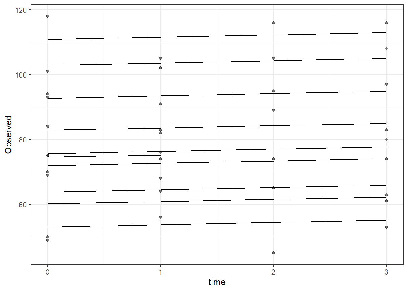
Fixed and Random effect of Time
fit <- lmer(Observed ~ 1 + time + (1 + time || SubjectID),
            data = mydata)
summary(fit)
Linear mixed model fit by REML. t-tests use Satterthwaite's method [
lmerModLmerTest]
Formula: Observed ~ 1 + time + (1 + time || SubjectID)
Data: mydata
REML criterion at convergence: 274.4
Scaled residuals:
Min 1Q Median 3Q Max
-2.8761 -0.3026 0.1033 0.4303 2.4972
Random effects:
Groups Name Variance Std.Dev.
SubjectID (Intercept) 343.84452 18.5430
SubjectID.1 time 0.02544 0.1595
Residual 49.18804 7.0134
Number of obs: 37, groups: SubjectID, 11
Fixed effects:
Estimate Std. Error df t value Pr(>|t|)
(Intercept) 79.9745 5.8771 10.8727 13.608 3.6e-08 ***
time 0.7044 1.0449 9.0362 0.674 0.517
---
Signif. codes: 0 '***' 0.001 '**' 0.01 '*' 0.05 '.' 0.1 ' ' 1
Correlation of Fixed Effects:
(Intr)
time -0.223ranova(fit) # can take out random effect timeANOVA-like table for random-effects: Single term deletions
Model:
Observed ~ time + (1 | SubjectID) + (0 + time | SubjectID)
npar logLik AIC LRT Df Pr(>Chisq)
<none> 5 -137.22 284.44
(1 | SubjectID) 4 -153.74 315.47 33.035 1 9.05e-09 ***
time in (0 + time | SubjectID) 4 -137.22 282.44 0.000 1 0.9962
---
Signif. codes: 0 '***' 0.001 '**' 0.01 '*' 0.05 '.' 0.1 ' ' 1plot(fit)
dat <- cbind(mydata, fit=predict(fit))

ggplot(dat, aes(time, Observed, group=SubjectID))+
  geom_line(aes(y=fit))+
  geom_point(alpha=0.5)#+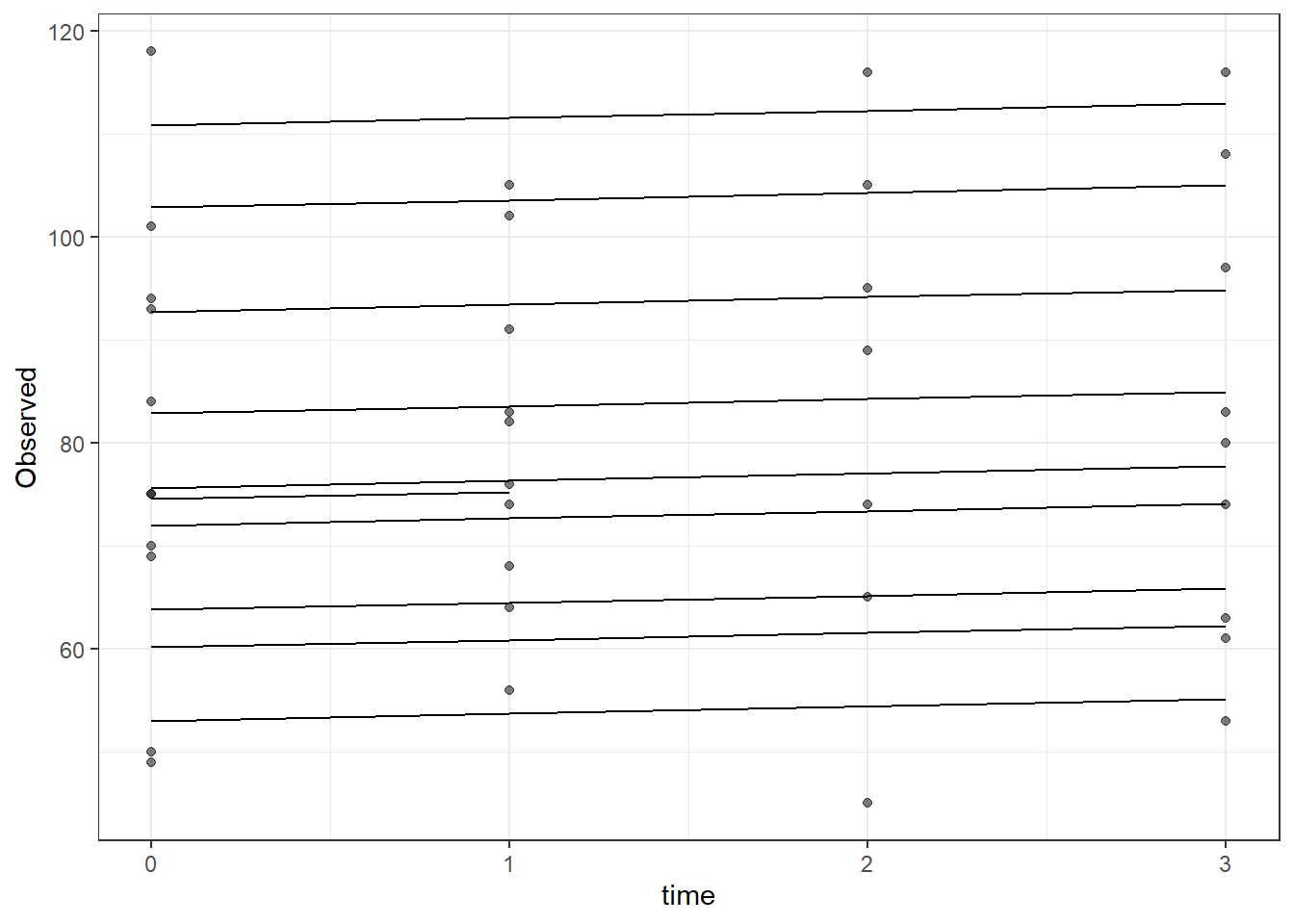
  #geom_abline(intercept = fixef(fit)[1], slope=fixef(fit)[2],
              #linetype="dashed", size=1.5)
Adding demographics
Time is only a fixed effect.
fit <- lmer(Observed ~ 1 + time + female + hispanic + (1 | SubjectID),
            data = mydata)
summary(fit)
Linear mixed model fit by REML. t-tests use Satterthwaite's method [
lmerModLmerTest]
Formula: Observed ~ 1 + time + female + hispanic + (1 | SubjectID)
Data: mydata
REML criterion at convergence: 260.1
Scaled residuals:
Min 1Q Median 3Q Max
-2.8378 -0.2979 0.1045 0.3988 2.5353
Random effects:
Groups Name Variance Std.Dev.
SubjectID (Intercept) 404.90 20.122
Residual 49.24 7.017
Number of obs: 37, groups: SubjectID, 11
Fixed effects:
Estimate Std. Error df t value Pr(>|t|)
(Intercept) 73.7523 12.2582 8.2397 6.017 0.000282 ***
time 0.7036 1.0451 25.3935 0.673 0.506875
female 9.4770 13.1744 8.0765 0.719 0.492215
hispanic 0.3278 13.1587 8.0384 0.025 0.980733
---
Signif. codes: 0 '***' 0.001 '**' 0.01 '*' 0.05 '.' 0.1 ' ' 1
Correlation of Fixed Effects:
(Intr) time female
time -0.118
female -0.537 -0.011
hispanic -0.537 0.028 -0.213ranova(fit)ANOVA-like table for random-effects: Single term deletions
Model:
Observed ~ time + female + hispanic + (1 | SubjectID)
npar logLik AIC LRT Df Pr(>Chisq)
<none> 6 -130.03 272.06
(1 | SubjectID) 5 -151.64 313.28 43.216 1 4.902e-11 ***
---
Signif. codes: 0 '***' 0.001 '**' 0.01 '*' 0.05 '.' 0.1 ' ' 1plot(fit)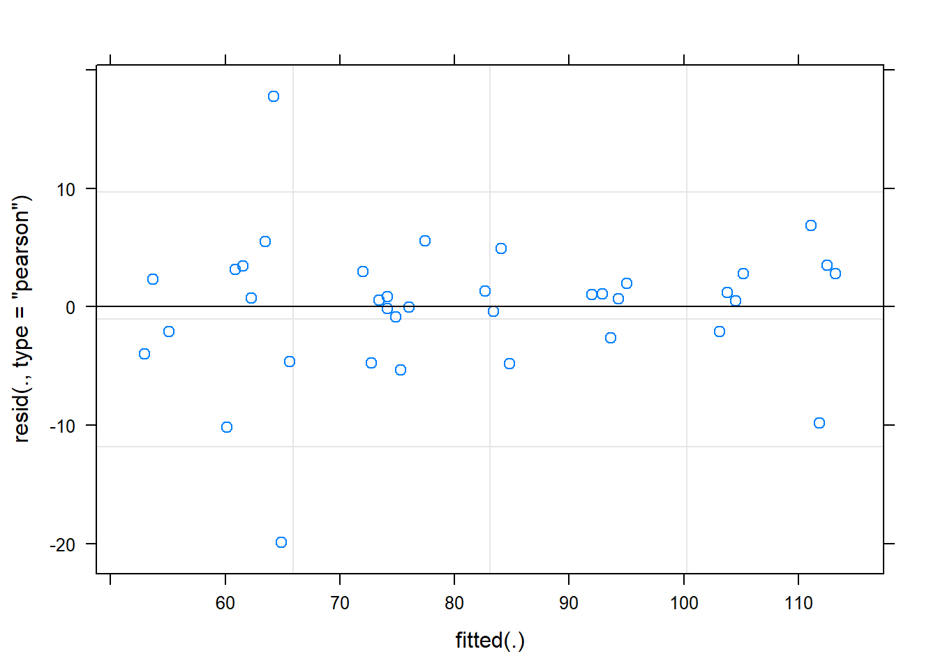
ICC(fit)[1] 0.8915756dat <- cbind(mydata, fit=predict(fit))
ggplot(dat, aes(time, Observed, group=SubjectID, color=Gender))+
geom_line(aes(y=fit))+
geom_point(alpha=0.5)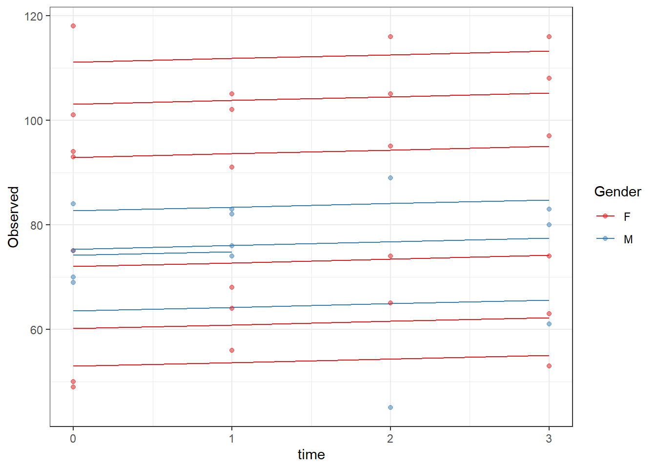
Intervention effect
fit <- lmer(Shannon ~ 1 + intB + time + female +  (1 | SubjectID),
            data = mydata)
summary(fit)
Linear mixed model fit by REML. t-tests use Satterthwaite's method [
lmerModLmerTest]
Formula: Shannon ~ 1 + intB + time + female + (1 | SubjectID)
Data: mydata
REML criterion at convergence: 32.1
Scaled residuals:
Min 1Q Median 3Q Max
-2.5421 -0.2129 0.0820 0.4446 2.3060
Random effects:
Groups Name Variance Std.Dev.
SubjectID (Intercept) 0.24559 0.4956
Residual 0.05679 0.2383
Number of obs: 37, groups: SubjectID, 11
Fixed effects:
Estimate Std. Error df t value Pr(>|t|)
(Intercept) 2.28187 0.30568 8.58797 7.465 4.93e-05 ***
intB 0.18778 0.31332 8.16541 0.599 0.565
time 0.02692 0.03539 25.65600 0.761 0.454
female 0.21545 0.32387 8.13481 0.665 0.524
---
Signif. codes: 0 '***' 0.001 '**' 0.01 '*' 0.05 '.' 0.1 ' ' 1
Correlation of Fixed Effects:
(Intr) intB time
intB -0.522
time -0.144 0.005
female -0.713 0.088 -0.007ranova(fit)ANOVA-like table for random-effects: Single term deletions
Model:
Shannon ~ intB + time + female + (1 | SubjectID)
npar logLik AIC LRT Df Pr(>Chisq)
<none> 6 -16.037 44.073
(1 | SubjectID) 5 -30.640 71.280 29.207 1 6.503e-08 ***
---
Signif. codes: 0 '***' 0.001 '**' 0.01 '*' 0.05 '.' 0.1 ' ' 1plot(fit)
ICC(fit)[1] 0.8121832dat <- cbind(mydata, fit=predict(fit))
ggplot(dat, aes(time, Shannon, group=SubjectID, color=Intervention))+
geom_line(aes(y=fit))+
geom_point(alpha=0.5)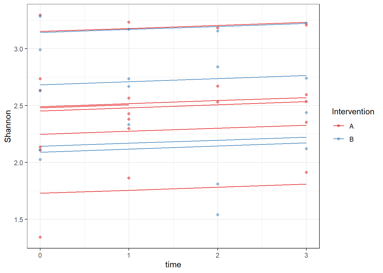
Overall Effect
fit <- lmer(Observed ~ 1 + intB + female + hispanic + (1 | SubjectID),
            data = mydata)
summary(fit)
Linear mixed model fit by REML. t-tests use Satterthwaite's method [
lmerModLmerTest]
Formula: Observed ~ 1 + intB + female + hispanic + (1 | SubjectID)
Data: mydata
REML criterion at convergence: 255.3
Scaled residuals:
Min 1Q Median 3Q Max
-2.8214 -0.4218 0.1150 0.4418 2.5037
Random effects:
Groups Name Variance Std.Dev.
SubjectID (Intercept) 455.39 21.340
Residual 48.28 6.948
Number of obs: 37, groups: SubjectID, 11
Fixed effects:
Estimate Std. Error df t value Pr(>|t|)
(Intercept) 73.151 13.678 7.089 5.348 0.00102 **
intB 4.797 14.012 7.130 0.342 0.74198
female 10.329 14.106 7.115 0.732 0.48746
hispanic -1.607 14.767 7.046 -0.109 0.91639
---
Signif. codes: 0 '***' 0.001 '**' 0.01 '*' 0.05 '.' 0.1 ' ' 1
Correlation of Fixed Effects:
(Intr) intB female
intB -0.337
female -0.557 0.155
hispanic -0.365 -0.334 -0.250plot(fit)
ICC(fit)[1] 0.9041487dat <- cbind(mydata, fit=predict(fit))
ggplot(dat, aes(time, Observed, group=SubjectID, color=Intervention))+
geom_line(aes(y=fit))+
geom_point(alpha=0.5)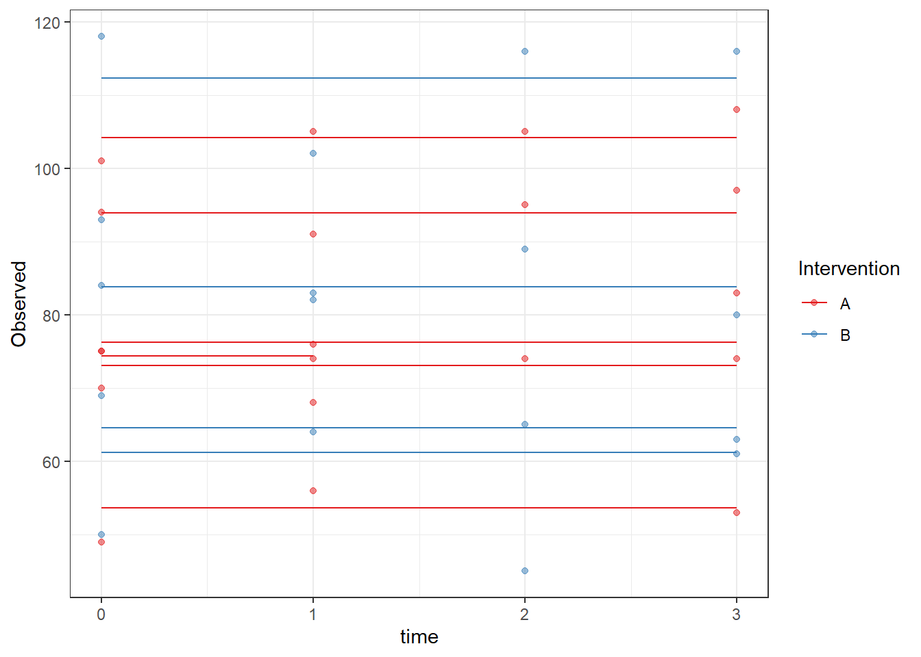
With Time
fit <- lmer(Observed ~ 1 + intB*time + (1 | SubjectID),
            data = mydata)
alpha.fit[["Observed"]]<- summary(fit)[["coefficients"]]
summary(fit)
Linear mixed model fit by REML. t-tests use Satterthwaite's method [
lmerModLmerTest]
Formula: Observed ~ 1 + intB * time + (1 | SubjectID)
Data: mydata
REML criterion at convergence: 263.1
Scaled residuals:
Min 1Q Median 3Q Max
-2.79078 -0.27419 0.04933 0.40138 2.41053
Random effects:
Groups Name Variance Std.Dev.
SubjectID (Intercept) 374.98 19.364
Residual 49.09 7.006
Number of obs: 37, groups: SubjectID, 11
Fixed effects:
Estimate Std. Error df t value Pr(>|t|)
(Intercept) 77.063 8.267 9.975 9.322 3.07e-06 ***
intB 6.391 12.279 10.030 0.520 0.614
time 1.733 1.403 24.342 1.235 0.229
intB:time -2.291 2.097 24.504 -1.093 0.285
---
Signif. codes: 0 '***' 0.001 '**' 0.01 '*' 0.05 '.' 0.1 ' ' 1
Correlation of Fixed Effects:
(Intr) intB time
intB -0.673
time -0.218 0.146
intB:time 0.146 -0.213 -0.669ranova(fit)ANOVA-like table for random-effects: Single term deletions
Model:
Observed ~ intB + time + (1 | SubjectID) + intB:time
npar logLik AIC LRT Df Pr(>Chisq)
<none> 6 -131.53 275.06
(1 | SubjectID) 5 -152.63 315.27 42.206 1 8.215e-11 ***
---
Signif. codes: 0 '***' 0.001 '**' 0.01 '*' 0.05 '.' 0.1 ' ' 1plot(fit)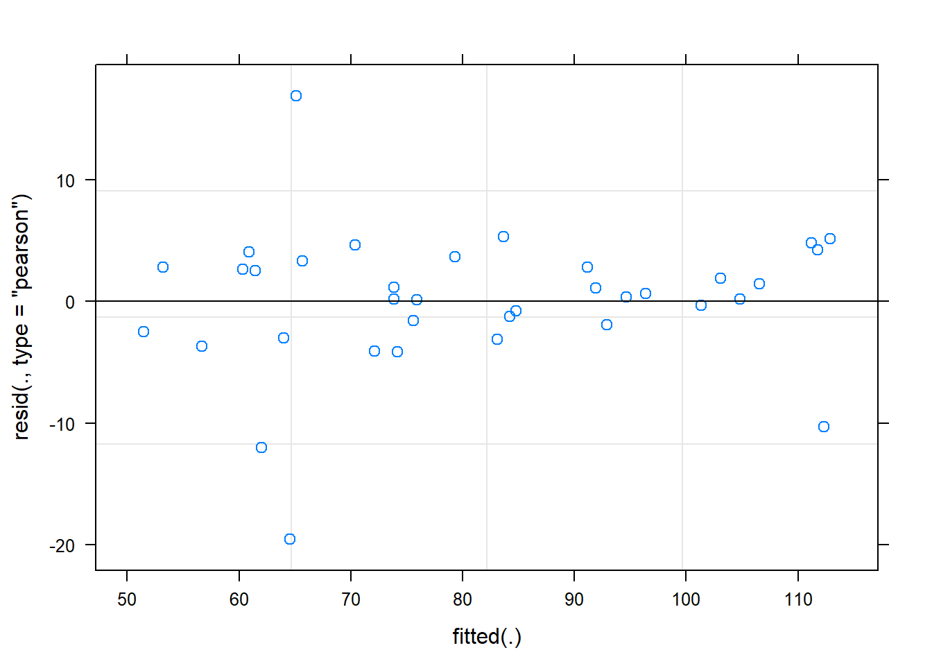
ICC(fit)[1] 0.8842445dat <- cbind(mydata, fit=predict(fit))
ggplot(dat, aes(time, Observed, group=SubjectID, color=Intervention))+
geom_line(aes(y=fit))+
geom_point(alpha=0.5)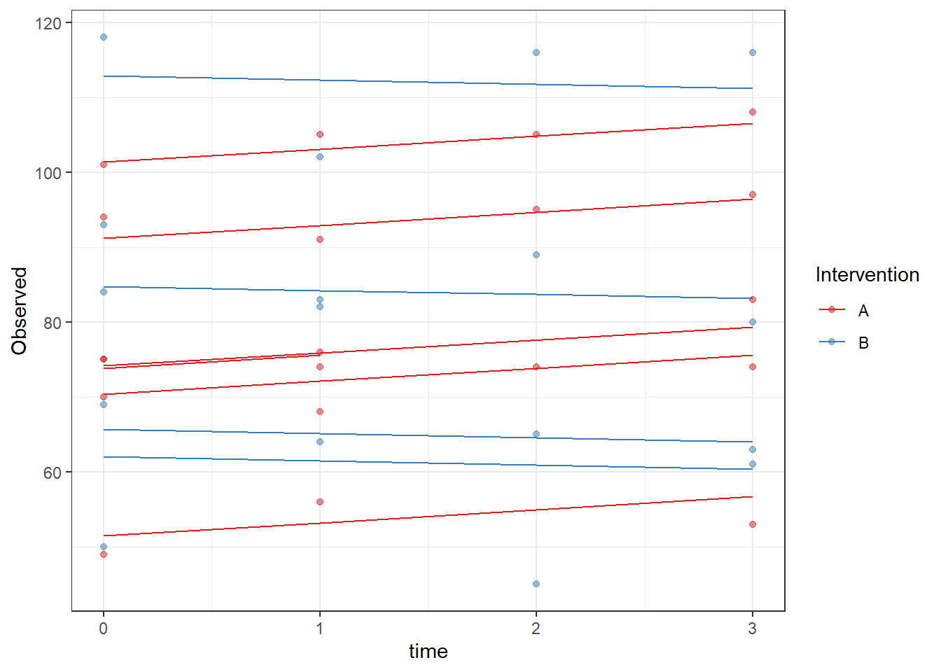
Alpha: Shannon Diversity
Unconditional Model
# lmer - for alpha metrics
# unconditional model
fit <- lmer(Shannon ~ 1 + (1 | SubjectID),
            data = mydata)
summary(fit)
Linear mixed model fit by REML. t-tests use Satterthwaite's method [
lmerModLmerTest]
Formula: Shannon ~ 1 + (1 | SubjectID)
Data: mydata
REML criterion at convergence: 27.5
Scaled residuals:
Min 1Q Median 3Q Max
-2.52108 -0.10901 0.09227 0.42858 2.24145
Random effects:
Groups Name Variance Std.Dev.
SubjectID (Intercept) 0.20910 0.4573
Residual 0.05614 0.2369
Number of obs: 37, groups: SubjectID, 11
Fixed effects:
Estimate Std. Error df t value Pr(>|t|)
(Intercept) 2.5369 0.1441 10.0567 17.6 6.93e-09 ***
---
Signif. codes: 0 '***' 0.001 '**' 0.01 '*' 0.05 '.' 0.1 ' ' 1plot(fit)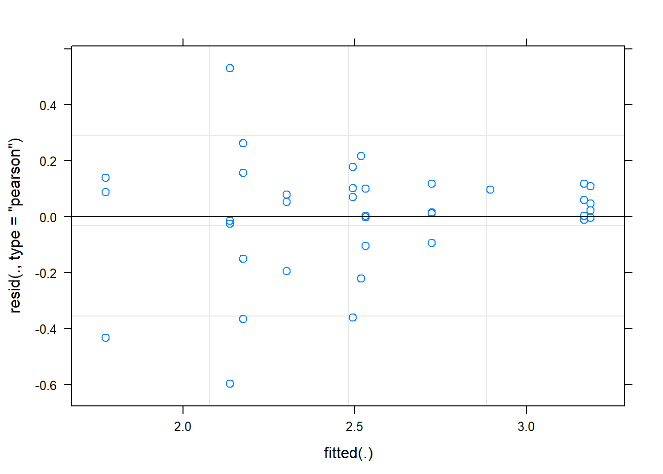
ICC(fit)[1] 0.7883435Fixed Effect of Time
fit <- lmer(Shannon ~ 1 + time + (1 | SubjectID),
            data = mydata)
summary(fit)
Linear mixed model fit by REML. t-tests use Satterthwaite's method [
lmerModLmerTest]
Formula: Shannon ~ 1 + time + (1 | SubjectID)
Data: mydata
REML criterion at convergence: 31.8
Scaled residuals:
Min 1Q Median 3Q Max
-2.56270 -0.23068 0.06454 0.43411 2.28067
Random effects:
Groups Name Variance Std.Dev.
SubjectID (Intercept) 0.21095 0.4593
Residual 0.05688 0.2385
Number of obs: 37, groups: SubjectID, 11
Fixed effects:
Estimate Std. Error df t value Pr(>|t|)
(Intercept) 2.50312 0.15156 12.01775 16.516 1.26e-09 ***
time 0.02671 0.03539 25.67099 0.755 0.457
---
Signif. codes: 0 '***' 0.001 '**' 0.01 '*' 0.05 '.' 0.1 ' ' 1
Correlation of Fixed Effects:
(Intr)
time -0.295plot(fit)
# plot
dat <- cbind(mydata, fit=predict(fit))
ggplot(dat, aes(time, Shannon, group=SubjectID))+
  geom_line(aes(y=fit))+
  geom_point(alpha=0.5)
Fixed and Random effect of Time
fit <- lmer(Shannon ~ 1 + time + (1 + time || SubjectID),
            data = mydata)
boundary (singular) fit: see ?isSingularsummary(fit)Linear mixed model fit by REML. t-tests use Satterthwaite's method [
lmerModLmerTest]
Formula: Shannon ~ 1 + time + (1 + time || SubjectID)
Data: mydata
REML criterion at convergence: 31.8
Scaled residuals:
Min 1Q Median 3Q Max
-2.56270 -0.23068 0.06454 0.43411 2.28067
Random effects:
Groups Name Variance Std.Dev.
SubjectID (Intercept) 0.21095 0.4593
SubjectID.1 time 0.00000 0.0000
Residual 0.05688 0.2385
Number of obs: 37, groups: SubjectID, 11
Fixed effects:
Estimate Std. Error df t value Pr(>|t|)
(Intercept) 2.50312 0.15156 12.01773 16.516 1.26e-09 ***
time 0.02671 0.03539 25.67099 0.755 0.457
---
Signif. codes: 0 '***' 0.001 '**' 0.01 '*' 0.05 '.' 0.1 ' ' 1
Correlation of Fixed Effects:
(Intr)
time -0.295
convergence code: 0
boundary (singular) fit: see ?isSingularranova(fit) # can take out random effect timeANOVA-like table for random-effects: Single term deletions
Model:
Shannon ~ time + (1 | SubjectID) + (0 + time | SubjectID)
npar logLik AIC LRT Df Pr(>Chisq)
<none> 5 -15.904 41.808
(1 | SubjectID) 4 -28.136 64.272 24.464 1 7.573e-07 ***
time in (0 + time | SubjectID) 4 -15.904 39.808 0.000 1 1
---
Signif. codes: 0 '***' 0.001 '**' 0.01 '*' 0.05 '.' 0.1 ' ' 1plot(fit)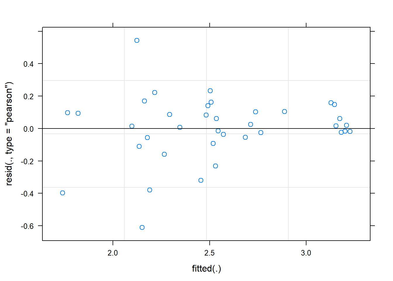
dat <- cbind(mydata, fit=predict(fit))

ggplot(dat, aes(time, Shannon, group=SubjectID))+
  geom_line(aes(y=fit))+
  geom_point(alpha=0.5)#+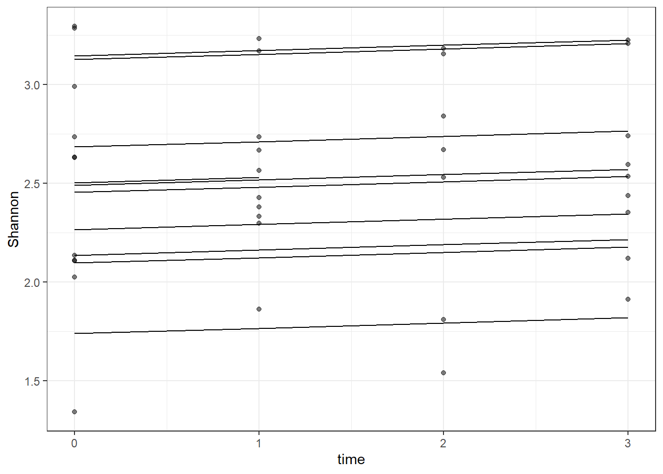
  #geom_abline(intercept = fixef(fit)[1], slope=fixef(fit)[2],
              #linetype="dashed", size=1.5)
Adding demographics
Time is only a fixed effect.
fit <- lmer(Shannon ~ 1 + time + female + hispanic + (1 | SubjectID),
            data = mydata)
summary(fit)
Linear mixed model fit by REML. t-tests use Satterthwaite's method [
lmerModLmerTest]
Formula: Shannon ~ 1 + time + female + hispanic + (1 | SubjectID)
Data: mydata
REML criterion at convergence: 32.3
Scaled residuals:
Min 1Q Median 3Q Max
-2.52044 -0.19196 0.07653 0.43541 2.32382
Random effects:
Groups Name Variance Std.Dev.
SubjectID (Intercept) 0.25601 0.5060
Residual 0.05687 0.2385
Number of obs: 37, groups: SubjectID, 11
Fixed effects:
Estimate Std. Error df t value Pr(>|t|)
(Intercept) 2.39623 0.31436 8.28622 7.623 5.11e-05 ***
time 0.02675 0.03545 25.53005 0.755 0.457
female 0.20648 0.33656 7.99580 0.613 0.557
hispanic -0.03743 0.33585 7.92920 -0.111 0.914
---
Signif. codes: 0 '***' 0.001 '**' 0.01 '*' 0.05 '.' 0.1 ' ' 1
Correlation of Fixed Effects:
(Intr) time female
time -0.156
female -0.535 -0.015
hispanic -0.535 0.036 -0.212ranova(fit)ANOVA-like table for random-effects: Single term deletions
Model:
Shannon ~ time + female + hispanic + (1 | SubjectID)
npar logLik AIC LRT Df Pr(>Chisq)
<none> 6 -16.157 44.313
(1 | SubjectID) 5 -30.816 71.632 29.319 1 6.138e-08 ***
---
Signif. codes: 0 '***' 0.001 '**' 0.01 '*' 0.05 '.' 0.1 ' ' 1plot(fit)
ICC(fit)[1] 0.818249dat <- cbind(mydata, fit=predict(fit))
ggplot(dat, aes(time, Shannon, group=SubjectID, color=Gender))+
geom_line(aes(y=fit))+
geom_point(alpha=0.5)
Intervention effect
fit <- lmer(Shannon ~ 1 + intB + time + female +  (1 | SubjectID),
            data = mydata)
summary(fit)
Linear mixed model fit by REML. t-tests use Satterthwaite's method [
lmerModLmerTest]
Formula: Shannon ~ 1 + intB + time + female + (1 | SubjectID)
Data: mydata
REML criterion at convergence: 32.1
Scaled residuals:
Min 1Q Median 3Q Max
-2.5421 -0.2129 0.0820 0.4446 2.3060
Random effects:
Groups Name Variance Std.Dev.
SubjectID (Intercept) 0.24559 0.4956
Residual 0.05679 0.2383
Number of obs: 37, groups: SubjectID, 11
Fixed effects:
Estimate Std. Error df t value Pr(>|t|)
(Intercept) 2.28187 0.30568 8.58797 7.465 4.93e-05 ***
intB 0.18778 0.31332 8.16541 0.599 0.565
time 0.02692 0.03539 25.65600 0.761 0.454
female 0.21545 0.32387 8.13481 0.665 0.524
---
Signif. codes: 0 '***' 0.001 '**' 0.01 '*' 0.05 '.' 0.1 ' ' 1
Correlation of Fixed Effects:
(Intr) intB time
intB -0.522
time -0.144 0.005
female -0.713 0.088 -0.007ranova(fit)ANOVA-like table for random-effects: Single term deletions
Model:
Shannon ~ intB + time + female + (1 | SubjectID)
npar logLik AIC LRT Df Pr(>Chisq)
<none> 6 -16.037 44.073
(1 | SubjectID) 5 -30.640 71.280 29.207 1 6.503e-08 ***
---
Signif. codes: 0 '***' 0.001 '**' 0.01 '*' 0.05 '.' 0.1 ' ' 1plot(fit)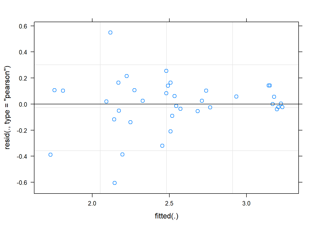
ICC(fit)[1] 0.8121832dat <- cbind(mydata, fit=predict(fit))
ggplot(dat, aes(time, Shannon, group=SubjectID, color=Intervention))+
geom_line(aes(y=fit))+
geom_point(alpha=0.5)
Overall Effect
fit <- lmer(Shannon ~ 1 + intB + female + hispanic + (1 | SubjectID),
            data = mydata)
summary(fit)
Linear mixed model fit by REML. t-tests use Satterthwaite's method [
lmerModLmerTest]
Formula: Shannon ~ 1 + intB + female + hispanic + (1 | SubjectID)
Data: mydata
REML criterion at convergence: 27.9
Scaled residuals:
Min 1Q Median 3Q Max
-2.50594 -0.11998 0.07058 0.42323 2.25810
Random effects:
Groups Name Variance Std.Dev.
SubjectID (Intercept) 0.27471 0.5241
Residual 0.05611 0.2369
Number of obs: 37, groups: SubjectID, 11
Fixed effects:
Estimate Std. Error df t value Pr(>|t|)
(Intercept) 2.3573 0.3414 7.0911 6.905 0.000217 ***
intB 0.2278 0.3501 7.1582 0.651 0.535667
female 0.2478 0.3523 7.1360 0.703 0.504195
hispanic -0.1264 0.3680 7.0115 -0.343 0.741353
---
Signif. codes: 0 '***' 0.001 '**' 0.01 '*' 0.05 '.' 0.1 ' ' 1
Correlation of Fixed Effects:
(Intr) intB female
intB -0.342
female -0.560 0.163
hispanic -0.360 -0.335 -0.251plot(fit)
ICC(fit)[1] 0.8304006dat <- cbind(mydata, fit=predict(fit))
ggplot(dat, aes(time, Shannon, group=SubjectID, color=Intervention))+
geom_line(aes(y=fit))+
geom_point(alpha=0.5)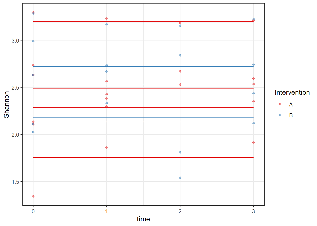
With Time
fit <- lmer(Shannon ~ 1 + intB*time + (1 | SubjectID),
            data = mydata)
alpha.fit[["Shannon"]]<- summary(fit)[["coefficients"]]
summary(fit)
Linear mixed model fit by REML. t-tests use Satterthwaite's method [
lmerModLmerTest]
Formula: Shannon ~ 1 + intB * time + (1 | SubjectID)
Data: mydata
REML criterion at convergence: 34.7
Scaled residuals:
Min 1Q Median 3Q Max
-2.49001 -0.30296 0.00711 0.43329 2.17948
Random effects:
Groups Name Variance Std.Dev.
SubjectID (Intercept) 0.2255 0.4748
Residual 0.0575 0.2398
Number of obs: 37, groups: SubjectID, 11
Fixed effects:
Estimate Std. Error df t value Pr(>|t|)
(Intercept) 2.38981 0.21075 10.75040 11.339 2.57e-07 ***
intB 0.24984 0.31339 10.84904 0.797 0.442
time 0.05601 0.04795 24.52409 1.168 0.254
intB:time -0.06478 0.07156 24.78004 -0.905 0.374
---
Signif. codes: 0 '***' 0.001 '**' 0.01 '*' 0.05 '.' 0.1 ' ' 1
Correlation of Fixed Effects:
(Intr) intB time
intB -0.672
time -0.292 0.197
intB:time 0.196 -0.287 -0.670ranova(fit)ANOVA-like table for random-effects: Single term deletions
Model:
Shannon ~ intB + time + (1 | SubjectID) + intB:time
npar logLik AIC LRT Df Pr(>Chisq)
<none> 6 -17.350 46.701
(1 | SubjectID) 5 -31.412 72.823 28.122 1 1.139e-07 ***
---
Signif. codes: 0 '***' 0.001 '**' 0.01 '*' 0.05 '.' 0.1 ' ' 1plot(fit)
ICC(fit)[1] 0.7968058dat <- cbind(mydata, fit=predict(fit))
ggplot(dat, aes(time, Shannon, group=SubjectID, color=Intervention))+
geom_line(aes(y=fit))+
geom_point(alpha=0.5)
Alpha: Inverse Simpson
Unconditional Model
# lmer - for alpha metrics
# unconditional model
fit <- lmer(InvSimpson ~ 1 + (1 | SubjectID),
            data = mydata)
summary(fit)
Linear mixed model fit by REML. t-tests use Satterthwaite's method [
lmerModLmerTest]
Formula: InvSimpson ~ 1 + (1 | SubjectID)
Data: mydata
REML criterion at convergence: 155
Scaled residuals:
Min 1Q Median 3Q Max
-1.52204 -0.77338 0.07031 0.50797 2.18754
Random effects:
Groups Name Variance Std.Dev.
SubjectID (Intercept) 13.503 3.675
Residual 1.552 1.246
Number of obs: 37, groups: SubjectID, 11
Fixed effects:
Estimate Std. Error df t value Pr(>|t|)
(Intercept) 7.081 1.130 9.950 6.266 9.52e-05 ***
---
Signif. codes: 0 '***' 0.001 '**' 0.01 '*' 0.05 '.' 0.1 ' ' 1plot(fit)
ICC(fit)[1] 0.8968883Fixed Effect of Time
fit <- lmer(InvSimpson ~ 1 + time + (1 | SubjectID),
            data = mydata)
summary(fit)
Linear mixed model fit by REML. t-tests use Satterthwaite's method [
lmerModLmerTest]
Formula: InvSimpson ~ 1 + time + (1 | SubjectID)
Data: mydata
REML criterion at convergence: 156.3
Scaled residuals:
Min 1Q Median 3Q Max
-1.46389 -0.85990 0.04318 0.47402 2.04966
Random effects:
Groups Name Variance Std.Dev.
SubjectID (Intercept) 13.421 3.663
Residual 1.602 1.266
Number of obs: 37, groups: SubjectID, 11
Fixed effects:
Estimate Std. Error df t value Pr(>|t|)
(Intercept) 7.19533 1.15194 10.84811 6.246 6.69e-05 ***
time -0.09191 0.18845 25.27704 -0.488 0.63
---
Signif. codes: 0 '***' 0.001 '**' 0.01 '*' 0.05 '.' 0.1 ' ' 1
Correlation of Fixed Effects:
(Intr)
time -0.205plot(fit)
# plot
dat <- cbind(mydata, fit=predict(fit))
ggplot(dat, aes(time, InvSimpson, group=SubjectID))+
  geom_line(aes(y=fit))+
  geom_point(alpha=0.5)
Fixed and Random effect of Time
fit <- lmer(InvSimpson ~ 1 + time + (1 + time || SubjectID),
            data = mydata)
boundary (singular) fit: see ?isSingularsummary(fit)Linear mixed model fit by REML. t-tests use Satterthwaite's method [
lmerModLmerTest]
Formula: InvSimpson ~ 1 + time + (1 + time || SubjectID)
Data: mydata
REML criterion at convergence: 156.3
Scaled residuals:
Min 1Q Median 3Q Max
-1.46389 -0.85990 0.04318 0.47402 2.04966
Random effects:
Groups Name Variance Std.Dev.
SubjectID (Intercept) 13.421 3.663
SubjectID.1 time 0.000 0.000
Residual 1.602 1.266
Number of obs: 37, groups: SubjectID, 11
Fixed effects:
Estimate Std. Error df t value Pr(>|t|)
(Intercept) 7.19533 1.15194 10.84811 6.246 6.69e-05 ***
time -0.09191 0.18845 25.27704 -0.488 0.63
---
Signif. codes: 0 '***' 0.001 '**' 0.01 '*' 0.05 '.' 0.1 ' ' 1
Correlation of Fixed Effects:
(Intr)
time -0.205
convergence code: 0
boundary (singular) fit: see ?isSingularranova(fit) # can take out random effect timeANOVA-like table for random-effects: Single term deletions
Model:
InvSimpson ~ time + (1 | SubjectID) + (0 + time | SubjectID)
npar logLik AIC LRT Df Pr(>Chisq)
<none> 5 -78.146 166.29
(1 | SubjectID) 4 -98.113 204.22 39.933 1 2.629e-10 ***
time in (0 + time | SubjectID) 4 -78.146 164.29 0.000 1 1
---
Signif. codes: 0 '***' 0.001 '**' 0.01 '*' 0.05 '.' 0.1 ' ' 1plot(fit)
dat <- cbind(mydata, fit=predict(fit))

ggplot(dat, aes(time, InvSimpson, group=SubjectID))+
  geom_line(aes(y=fit))+
  geom_point(alpha=0.5)#+
  #geom_abline(intercept = fixef(fit)[1], slope=fixef(fit)[2],
              #linetype="dashed", size=1.5)
Adding demographics
Time is only a fixed effect.
fit <- lmer(InvSimpson ~ 1 + time + female + hispanic + (1 | SubjectID),
            data = mydata)
summary(fit)
Linear mixed model fit by REML. t-tests use Satterthwaite's method [
lmerModLmerTest]
Formula: InvSimpson ~ 1 + time + female + hispanic + (1 | SubjectID)
Data: mydata
REML criterion at convergence: 147.8
Scaled residuals:
Min 1Q Median 3Q Max
-1.4312 -0.8217 0.0817 0.4629 2.0224
Random effects:
Groups Name Variance Std.Dev.
SubjectID (Intercept) 14.587 3.819
Residual 1.601 1.265
Number of obs: 37, groups: SubjectID, 11
Fixed effects:
Estimate Std. Error df t value Pr(>|t|)
(Intercept) 5.90971 2.32113 8.11406 2.546 0.034 *
time -0.09369 0.18847 25.26016 -0.497 0.623
female 2.78929 2.49580 7.96787 1.118 0.296
hispanic -0.76318 2.49310 7.93358 -0.306 0.767
---
Signif. codes: 0 '***' 0.001 '**' 0.01 '*' 0.05 '.' 0.1 ' ' 1
Correlation of Fixed Effects:
(Intr) time female
time -0.113
female -0.538 -0.010
hispanic -0.537 0.027 -0.213ranova(fit)ANOVA-like table for random-effects: Single term deletions
Model:
InvSimpson ~ time + female + hispanic + (1 | SubjectID)
npar logLik AIC LRT Df Pr(>Chisq)
<none> 6 -73.892 159.78
(1 | SubjectID) 5 -95.819 201.64 43.853 1 3.539e-11 ***
---
Signif. codes: 0 '***' 0.001 '**' 0.01 '*' 0.05 '.' 0.1 ' ' 1plot(fit)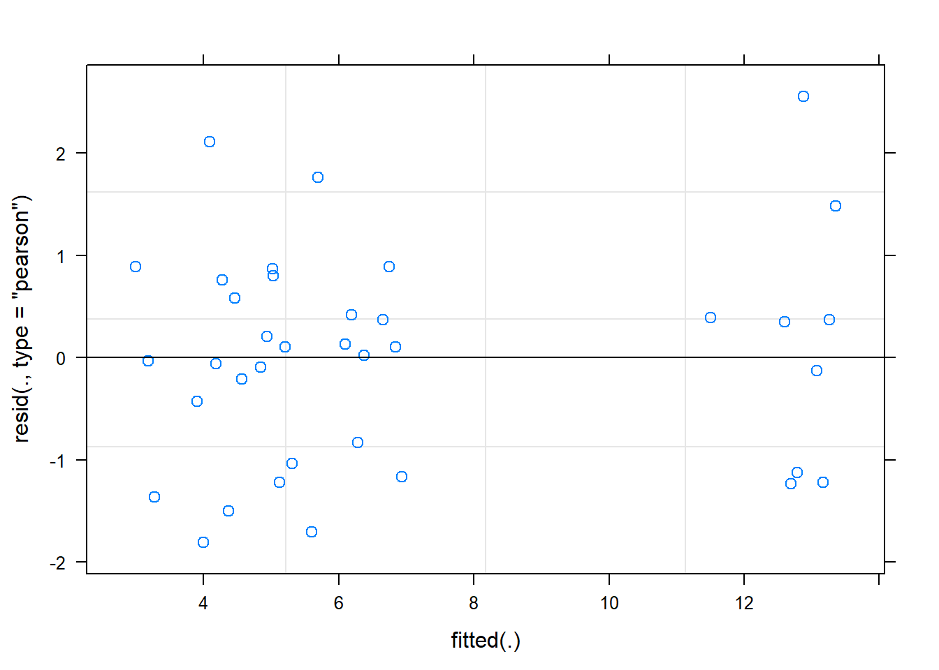
ICC(fit)[1] 0.9011189dat <- cbind(mydata, fit=predict(fit))
ggplot(dat, aes(time, InvSimpson, group=SubjectID, color=Gender))+
geom_line(aes(y=fit))+
geom_point(alpha=0.5)
Intervention effect
fit <- lmer(InvSimpson ~ 1 + intB + time + female +  (1 | SubjectID),
            data = mydata)
summary(fit)
Linear mixed model fit by REML. t-tests use Satterthwaite's method [
lmerModLmerTest]
Formula: InvSimpson ~ 1 + intB + time + female + (1 | SubjectID)
Data: mydata
REML criterion at convergence: 147.4
Scaled residuals:
Min 1Q Median 3Q Max
-1.44574 -0.78429 0.05668 0.43243 2.00430
Random effects:
Groups Name Variance Std.Dev.
SubjectID (Intercept) 13.788 3.713
Residual 1.598 1.264
Number of obs: 37, groups: SubjectID, 11
Fixed effects:
Estimate Std. Error df t value Pr(>|t|)
(Intercept) 4.64370 2.23242 8.31126 2.080 0.0698 .
intB 1.75177 2.30189 8.09859 0.761 0.4682
time -0.09201 0.18825 25.36968 -0.489 0.6292
female 2.76847 2.38072 8.07615 1.163 0.2781
---
Signif. codes: 0 '***' 0.001 '**' 0.01 '*' 0.05 '.' 0.1 ' ' 1
Correlation of Fixed Effects:
(Intr) intB time
intB -0.521
time -0.105 0.005
female -0.714 0.079 -0.005ranova(fit)ANOVA-like table for random-effects: Single term deletions
Model:
InvSimpson ~ intB + time + female + (1 | SubjectID)
npar logLik AIC LRT Df Pr(>Chisq)
<none> 6 -73.711 159.42
(1 | SubjectID) 5 -95.729 201.46 44.037 1 3.223e-11 ***
---
Signif. codes: 0 '***' 0.001 '**' 0.01 '*' 0.05 '.' 0.1 ' ' 1plot(fit)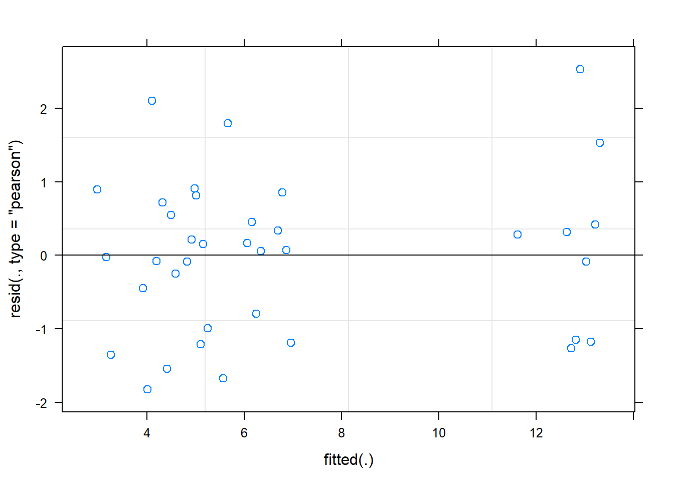
ICC(fit)[1] 0.8961121dat <- cbind(mydata, fit=predict(fit))
ggplot(dat, aes(time, InvSimpson, group=SubjectID, color=Intervention))+
geom_line(aes(y=fit))+
geom_point(alpha=0.5)
Overall Effect
fit <- lmer(InvSimpson ~ 1 + intB + female + hispanic + (1 | SubjectID),
            data = mydata)
summary(fit)
Linear mixed model fit by REML. t-tests use Satterthwaite's method [
lmerModLmerTest]
Formula: InvSimpson ~ 1 + intB + female + hispanic + (1 | SubjectID)
Data: mydata
REML criterion at convergence: 142
Scaled residuals:
Min 1Q Median 3Q Max
-1.5198 -0.7140 0.1027 0.4791 2.1389
Random effects:
Groups Name Variance Std.Dev.
SubjectID (Intercept) 15.21 3.900
Residual 1.55 1.245
Number of obs: 37, groups: SubjectID, 11
Fixed effects:
Estimate Std. Error df t value Pr(>|t|)
(Intercept) 5.041 2.498 7.028 2.018 0.0832 .
intB 2.244 2.559 7.068 0.877 0.4093
female 3.128 2.576 7.053 1.214 0.2638
hispanic -1.518 2.697 6.986 -0.563 0.5910
---
Signif. codes: 0 '***' 0.001 '**' 0.01 '*' 0.05 '.' 0.1 ' ' 1
Correlation of Fixed Effects:
(Intr) intB female
intB -0.337
female -0.556 0.155
hispanic -0.365 -0.334 -0.250plot(fit)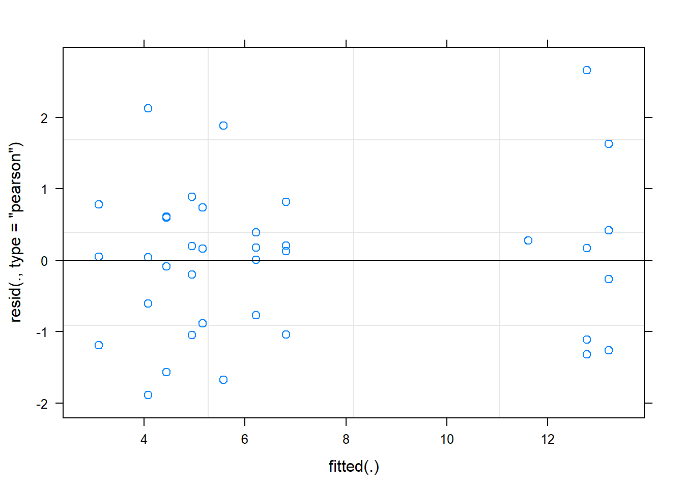
ICC(fit)[1] 0.9075388dat <- cbind(mydata, fit=predict(fit))
ggplot(dat, aes(time, InvSimpson, group=SubjectID, color=Intervention))+
geom_line(aes(y=fit))+
geom_point(alpha=0.5)
With Time
fit <- lmer(InvSimpson ~ 1 + intB*time + (1 | SubjectID),
            data = mydata)
alpha.fit[["InvSimpson"]]<- summary(fit)[["coefficients"]]
summary(fit)
Linear mixed model fit by REML. t-tests use Satterthwaite's method [
lmerModLmerTest]
Formula: InvSimpson ~ 1 + intB * time + (1 | SubjectID)
Data: mydata
REML criterion at convergence: 151.8
Scaled residuals:
Min 1Q Median 3Q Max
-1.44162 -0.68525 0.04353 0.47400 1.81068
Random effects:
Groups Name Variance Std.Dev.
SubjectID (Intercept) 14.087 3.753
Residual 1.631 1.277
Number of obs: 37, groups: SubjectID, 11
Fixed effects:
Estimate Std. Error df t value Pr(>|t|)
(Intercept) 6.32090 1.59436 9.77178 3.965 0.00279 **
intB 1.92485 2.36789 9.82030 0.813 0.43554
time 0.04721 0.25587 24.21942 0.185 0.85514
intB:time -0.30876 0.38244 24.36731 -0.807 0.42728
---
Signif. codes: 0 '***' 0.001 '**' 0.01 '*' 0.05 '.' 0.1 ' ' 1
Correlation of Fixed Effects:
(Intr) intB time
intB -0.673
time -0.206 0.138
intB:time 0.138 -0.201 -0.669ranova(fit)ANOVA-like table for random-effects: Single term deletions
Model:
InvSimpson ~ intB + time + (1 | SubjectID) + intB:time
npar logLik AIC LRT Df Pr(>Chisq)
<none> 6 -75.889 163.78
(1 | SubjectID) 5 -97.772 205.54 43.765 1 3.702e-11 ***
---
Signif. codes: 0 '***' 0.001 '**' 0.01 '*' 0.05 '.' 0.1 ' ' 1plot(fit)
ICC(fit)[1] 0.8962229dat <- cbind(mydata, fit=predict(fit))
ggplot(dat, aes(time, InvSimpson, group=SubjectID, color=Intervention))+
geom_line(aes(y=fit))+
geom_point(alpha=0.5)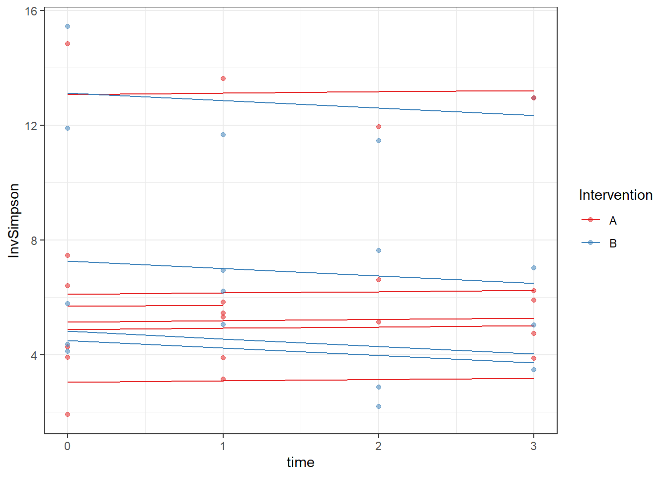
Summary of Results
To recap, the final model tested for which will have reported results in the manuscript is a growth model of each alpha diversity metric. The final growth model had the following form:
\[\begin{align*} Y_{ij}&=\beta_{0j} + \beta_{1j}(Week)_{ij} + r_{ij}\\ \beta_{0j}&= \gamma_{00} + \gamma_{01}(Intervention)_{j} + u_{0j}\\ \beta_{1j}&= \gamma_{10} + \gamma_{11}(Intervention)_{j}\\ \end{align*}\] where, the major aim was to assess the significance of two terms:
- the main effect of the intervention on the intercept - indicating average changes in alpha diversity between intervention groups.
- the interaction between time and intervention (intB:time), which assessing the magnitude of the change in alpha diversity as the intervention progresses.
alpha.results <- unlist_results(alpha.fit)Joining, by = c("Metric", "Term", "Estimate", "Std. Error", "df", "t value", "Pr(>|t|)")
Joining, by = c("Metric", "Term", "Estimate", "Std. Error", "df", "t value", "Pr(>|t|)")kable(alpha.results, format="html", digits=3)%>%
kable_styling(full_width = T)| Metric | Term | Estimate | Std. Error | df | t value | Pr(>|t|) | p.adjust |
|---|---|---|---|---|---|---|---|
| Observed | intB | 6.391 | 12.279 | 10.030 | 0.520 | 0.614 | 0.691 |
| Observed | time | 1.733 | 1.403 | 24.342 | 1.235 | 0.229 | 0.569 |
| Observed | intB:time | -2.291 | 2.097 | 24.504 | -1.093 | 0.285 | 0.569 |
| Shannon | intB | 0.250 | 0.313 | 10.849 | 0.797 | 0.442 | 0.569 |
| Shannon | time | 0.056 | 0.048 | 24.524 | 1.168 | 0.254 | 0.569 |
| Shannon | intB:time | -0.065 | 0.072 | 24.780 | -0.905 | 0.374 | 0.569 |
| InvSimpson | intB | 1.925 | 2.368 | 9.820 | 0.813 | 0.436 | 0.569 |
| InvSimpson | time | 0.047 | 0.256 | 24.219 | 0.185 | 0.855 | 0.855 |
| InvSimpson | intB:time | -0.309 | 0.382 | 24.367 | -0.807 | 0.427 | 0.569 |
Therefore, the intervention did not have a statistically significant effect on alpha diversity metrics.
sessionInfo()R version 3.6.3 (2020-02-29)
Platform: x86_64-w64-mingw32/x64 (64-bit)
Running under: Windows 10 x64 (build 18362)
Matrix products: default
locale:
[1] LC_COLLATE=English_United States.1252
[2] LC_CTYPE=English_United States.1252
[3] LC_MONETARY=English_United States.1252
[4] LC_NUMERIC=C
[5] LC_TIME=English_United States.1252
attached base packages:
[1] stats graphics grDevices utils datasets methods base
other attached packages:
[1] cowplot_1.0.0 microbiome_1.8.0 car_3.0-8 carData_3.0-4
[5] gvlma_1.0.0.3 patchwork_1.0.0 viridis_0.5.1 viridisLite_0.3.0
[9] gridExtra_2.3 xtable_1.8-4 kableExtra_1.1.0 plyr_1.8.6
[13] data.table_1.12.8 readxl_1.3.1 forcats_0.5.0 stringr_1.4.0
[17] dplyr_0.8.5 purrr_0.3.4 readr_1.3.1 tidyr_1.1.0
[21] tibble_3.0.1 ggplot2_3.3.0 tidyverse_1.3.0 lmerTest_3.1-2
[25] lme4_1.1-23 Matrix_1.2-18 vegan_2.5-6 lattice_0.20-38
[29] permute_0.9-5 phyloseq_1.30.0
loaded via a namespace (and not attached):
[1] Rtsne_0.15 minqa_1.2.4 colorspace_1.4-1
[4] rio_0.5.16 ellipsis_0.3.1 rprojroot_1.3-2
[7] XVector_0.26.0 fs_1.4.1 rstudioapi_0.11
[10] farver_2.0.3 fansi_0.4.1 lubridate_1.7.8
[13] xml2_1.3.2 codetools_0.2-16 splines_3.6.3
[16] knitr_1.28 ade4_1.7-15 jsonlite_1.6.1
[19] workflowr_1.6.2 nloptr_1.2.2.1 broom_0.5.6
[22] cluster_2.1.0 dbplyr_1.4.4 BiocManager_1.30.10
[25] compiler_3.6.3 httr_1.4.1 backports_1.1.7
[28] assertthat_0.2.1 cli_2.0.2 later_1.0.0
[31] htmltools_0.4.0 tools_3.6.3 igraph_1.2.5
[34] gtable_0.3.0 glue_1.4.1 reshape2_1.4.4
[37] Rcpp_1.0.4.6 Biobase_2.46.0 cellranger_1.1.0
[40] vctrs_0.3.0 Biostrings_2.54.0 multtest_2.42.0
[43] ape_5.3 nlme_3.1-144 iterators_1.0.12
[46] xfun_0.14 openxlsx_4.1.5 rvest_0.3.5
[49] lifecycle_0.2.0 statmod_1.4.34 zlibbioc_1.32.0
[52] MASS_7.3-51.5 scales_1.1.1 hms_0.5.3
[55] promises_1.1.0 parallel_3.6.3 biomformat_1.14.0
[58] rhdf5_2.30.1 RColorBrewer_1.1-2 curl_4.3
[61] yaml_2.2.1 stringi_1.4.6 highr_0.8
[64] S4Vectors_0.24.4 foreach_1.5.0 BiocGenerics_0.32.0
[67] zip_2.0.4 boot_1.3-24 rlang_0.4.6
[70] pkgconfig_2.0.3 evaluate_0.14 Rhdf5lib_1.8.0
[73] labeling_0.3 tidyselect_1.1.0 magrittr_1.5
[76] R6_2.4.1 IRanges_2.20.2 generics_0.0.2
[79] DBI_1.1.0 foreign_0.8-75 pillar_1.4.4
[82] haven_2.3.0 whisker_0.4 withr_2.2.0
[85] mgcv_1.8-31 abind_1.4-5 survival_3.1-8
[88] modelr_0.1.8 crayon_1.3.4 rmarkdown_2.1
[91] grid_3.6.3 blob_1.2.1 git2r_0.27.1
[94] reprex_0.3.0 digest_0.6.25 webshot_0.5.2
[97] httpuv_1.5.2 numDeriv_2016.8-1.1 stats4_3.6.3
[100] munsell_0.5.0